

Keras is a high-level neural network API written in Python.
This means that Keras abstracts away a lot of the complexity in building a deep neural network.
Keras provides us with a simple interface to rapidly build, test, and deploy deep learning architectures.
Because of this, Keras is by far the best learning tool for beginners in machine learning, as well as for experienced practitioners looking to quickly prototype a model.
Keras is also capable of running on top of other deep learning frameworks like TensorFlow, CNTK, and Theano.
In this article, we'll provide a step-by-step tutorial for building your first neural network in Python with Keras.
For the backend computation engine we will use TensorFlow.
We will first cover what is often referred to as the "Hello, World!" of CNNs—training a neural network that recognizes handwritten digits from the MNIST database.

We will then look at a slightly more challenging dataset: the Fashion MNIST Dataset.
The Fashion MNIST dataset was created by the eCommerce company Zalando.
As they describe on the Github repository, the reasons they created this dataset include:
- MNIST is too easy - as you'll see with the convolutional neural network below, it is quite easy to get the model to achieve a 99%+ accuracy
- MNIST is overused
- MNIST can not represent modern computer vision tasks
Zalando created the Fashion MNIST dataset as a replacement for MNIST.

Before we get into the code, let's first define the machine learning problem we are trying to solve.
Stay up to date with AI
The MNIST Dataset
Defining Our Machine Learning Problem
As mentioned, we'll be training a neural network that recognizes handwritten digits from the MNIST database, which is a publicly available dataset that consists of images of hand-written single digits.
Each image is a 28 by 28 pixel square, which means each has 784 total pixels.
We will use the standard split of the dataset, which is 60,000 images for training our model and 10,000 for testing our model.
The goal is to recognize handwritten digits, which means we have 10 classes to predict (0 to 9).
Our goal will be to train the neural network to achieve less than 1% prediction error, or 99%+ accuracy.
Loading Our Data
To build this neural network we will be using the free cloud-based, GPU-enabled Jupyter notebook environment: Google Colab.
Let's start by importing the MNIST dataset, which is conveniently provided by the Keras library.
We'll also import the classes and functions we'll need:
import kerasfrom keras.datasets
import mnistfrom keras.models
import Sequential
from keras.layers import Dense, Dropout, Flatten, Activation
from keras.layers import Conv2D, MaxPooling2D
from keras import backend as K
We'll then split the data between training and testing sets:
(X_train, y_train), (X_test, y_test) = mnist.load_data()Next, we'll import Matplotlib for data visualization and plot the first 2 images in the training dataset.
# import matplotlib for visualization
import matplotlib.pyplot as plt

# plot 2 images as gray scale
plt.subplot(221)plt.imshow(X_train[0], cmap=plt.get_cmap('gray'))
plt.subplot(222)plt.imshow(X_train[1], cmap=plt.get_cmap('gray'));
Preparing Our Data
We will start by setting the model's tuning parameters as follows:
batch_size = 128
num_classes = 10
epochs = 12
Next, we will flatten our dataset from images that are structured as 28 by 28 pixels to a vector that has 784 pixel input values.
We will first input our image dimensions.
# input image dimensions
img_rows, img_cols = 28, 28
And then we reshape our data.
We will also normalize the pixel values from grayscale, which are between 0 and 255 to a range between 0 and 1. We do this by dividing each by 255:
if K.image_data_format() == 'channels_first':
    X_train = X_train.reshape(X_train.shape[0], 1, img_rows, img_cols)
    X_test = X_test.reshape(X_test.shape[0], 1, img_rows, img_cols)
    input_shape = (1, img_rows, img_cols)
else:
    X_train = X_train.reshape(X_train.shape[0], img_rows, img_cols, 1)
    X_test = X_test.reshape(X_test.shape[0], img_rows, img_cols, 1)
    input_shape = (img_rows, img_cols, 1)

X_train = X_train.astype('float32')
X_test = X_test.astype('float32')
X_train /= 255
X_test /= 255
print('X_train shape:', X_train.shape)
print(X_train.shape[0], 'training samples')
print(X_test.shape[0], 'testing samples')
In order to make this data understandable by our neural network, it is good practice to apply one hot encoding.
Since this is a multi-class (0-9) classification problem, this will convert the class vectors into binary class matrices.
For example, let's say the digit is a 2 we will convert the vector from [0 1 2 3 4 5 6 7 8 9] to [0 0 1 0 0 0 0 0 0 0].
We will use the built-in utils.to_categorical() function that Keras provides.
y_train = keras.utils.to_categorical(y_train, num_classes)
y_test = keras.utils.to_categorical(y_test, num_classes)
Defining Our Neural Network
We will now define our neural network model, which as mentioned will use TensorFlow as the model's backend.
The structure of our convolutional neural network architecture is defined below:
- The first hidden layer
Conv2Dis a convolutional layer that has 32 feature maps, each with a size of 3 x 3 and we are using a rectified linear activation function -relu. - We then add another convolutional layer with 64 feature maps
- We add a third convolutional layer with 128 feature maps
- We then add a pooling layer
MaxPooling2D1that is configured with a pool size of 2 x 2 - We then apply a regularization layer using
Dropoutthat is set to randomly exclude 25% of the neurons in the layer - this is used to reduce overfitting - We then convert the 2-dimensional matrix into a vector using
Flatten- this allows our output to be processed by fully connected layers - Next, we add a fully connected layer that has 128 neurons and a ReLU activation function
- We will then add another regularization layer to reduce overfitting, this time we're randomly excluding 50% of the neurons
- We finish the neural network with an output layer that has 10 neurons - the same as the number of classes in our classification problem and a softmax activation function. This will output a prediction of the probability that a digit belongs to each class.
# import TensorFlow backend
import tensorflow as tf

# define our model
model = Sequential()
model = Sequential()
model.add(Conv2D(32, kernel_size=(3, 3), activation='relu',input_shape=input_shape))
model.add(Conv2D(64, (3, 3), activation='relu'))
model.add(Conv2D(128, (3, 3), activation='relu'))
model.add(MaxPooling2D(pool_size=(2, 2)))
model.add(Dropout(0.25))
model.add(Flatten())
model.add(Dense(128, activation='relu'))
model.add(Dropout(0.5))
model.add(Dense(num_classes, activation=Activation(tf.nn.softmax)))
Compiling the Model
We will then compile our model using a logarithmic loss and the Adadelta optimizer, which:
...adapts learning rates based on a moving window of gradient updates, instead of accumulating all past gradients. This way, Adadelta continues learning even when many updates have been done.
model.compile(loss=keras.losses.categorical_crossentropy,
		optimizer=keras.optimizers.Adadelta(), metrics=['accuracy'])
Train the Model
We will now fit the model using our batch size of 128 and 12 epochs.
model.fit(X_train, y_train, batch_size=batch_size, epochs=epochs,
		verbose=1, validation_data=(X_test, y_test))
Evaluating the Model
Finally, we will evaluate our model and print the accuracy:
score = model.evaluate(X_test, y_test, verbose=0)
print('Test Loss:', score[0])
print('Test Accuracy:', score[1])
Fashion MNIST with Keras
The Fashion MNIST dataset is identical to the MNIST dataset in terms of training size, testing size, the number of class labels, and image dimensions.
To recap, the dataset has:
- 60,000 training examples
- 10,000 testing examples
- 10 classes
- 28×28 grayscale images
The 10 classes for this dataset include:

Since we already have a CNN that works well with this dataset, we will first see if we can just change a few lines of code and still achieve high accuracy.
Let's start by importing the following packages:
import kerasfrom keras.datasets
import fashion_mnistfrom keras.models
import Sequentialfrom keras.layers
import Dense, Dropout, Flatten, Activation
from keras.layers import Conv2D, MaxPooling2D
from keras import backend as Kimport tensorflow as tf
We'll then download the Fashion MNIST dataset, which is also conveniently provided by the Keras library.
(X_train, y_train), (X_test, y_test) = fashion_mnist.load_data()Data Visualization
Let's now take a look at the first two images in the dataset:
# import matplotlib for visualization
import matplotlib.pyplot as plt

# plot 2 images as gray scale
plt.subplot(221)
plt.imshow(X_train[0], cmap=plt.get_cmap('gray'))
plt.subplot(222)
plt.imshow(X_train[1], cmap=plt.get_cmap('gray'));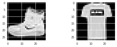
After that everything will be the same as our original model:
Set Tuning Parameters
# tuning parameters
batch_size = 128
num_classes = 10
epochs = 12
Input Image Dimensions
# input image dimensions
img_rows, img_cols = 28, 28
Reshape the Data
# reshape our datai
f K.image_data_format() == 'channels_first':
	X_train = X_train.reshape(X_train.shape[0], 1, img_rows, img_cols)
    X_test = X_test.reshape(X_test.shape[0], 1, img_rows, img_cols)
    input_shape = (1, img_rows, img_cols)
else:
	X_train = X_train.reshape(X_train.shape[0], img_rows, img_cols, 1)
    X_test = X_test.reshape(X_test.shape[0], img_rows, img_cols, 1
    input_shape = (img_rows, img_cols, 1)

X_train = X_train.astype('float32')
X_test = X_test.astype('float32')
X_train /= 255
X_test /= 255
print('X_train shape:', X_train.shape)
print(X_train.shape[0], 'training samples')
print(X_test.shape[0], 'testing samples')
Apply One Hot Encoding to the Data
y_train = keras.utils.to_categorical(y_train, num_classes)
y_test = keras.utils.to_categorical(y_test, num_classes)
Create the Neural Network
model = Sequential()

#Add Layers to the Neural Network
model.add(Conv2D(32, kernel_size=(3, 3), activation='relu', input_shape=input_shape))
model.add(Conv2D(64, (3, 3), activation='relu'))
model.add(Conv2D(128, (3, 3), activation='relu'))
model.add(MaxPooling2D(pool_size=(2, 2)))
model.add(Dropout(0.25))
model.add(Flatten())
model.add(Dense(128, activation='relu'))
model.add(Dropout(0.5))
model.add(Dense(num_classes, activation=Activation(tf.nn.softmax)))
Compile the Model
model.compile(loss=keras.losses.categorical_crossentropy, optimizer=keras.optimizers.Adadelta(), metrics=['accuracy'])Train the Model
model.fit(X_train, y_train, batch_size=batch_size, epochs=epochs, verbose=1, validation_data=(X_test, y_test))Evaluate the Results
score = model.evaluate(X_test, y_test, verbose=0)
print('Test Loss:', score[0])
print('Test Accuracy:', score[1])
As we can see this model achieves a 92.66% accuracy.
Let's see if we can improve that by tuning our models hyperparameters.
Hyperparameter Tuning
To start we will just increase the number of epochs to 48 and see how that does.
After evaluating the results we see that this model got 93.27% accuracy after 48 epochs, a slight increase in performance.
Other hyperparameters to tune that may increase performance include:
- Changing the learning rate
- Changing the optimizer from Adadelta
Summary: How to Build a CNN in Python with Keras
In this tutorial, we took our first steps in building a convolutional neural network with Keras and Python. We first looked at the MNIST database—the goal was to correctly classify handwritten digits, and as you can see we achieved a 99.19% accuracy for our model.
We then look at the Fashion MNIST dataset, a slightly more challenging dataset.
The goal was to correctly classify articles of clothing, and as we saw achieved a 93.27% accuracy.
To summarize, the steps we went through include:
- How to load a dataset in Keras
- How to prepare our data for training by reshaping it
- How to build a convolutional neural network
- How to train the model in Google Colab using a GPU-enabled processor
- How to evaluate our model
- How to tune our model's hyperparameters


