

In this article, we cover two important concepts in the field of reinforcement learning: Q-learning and deep Q-learning.
This article is based on the Deep Reinforcement Learning 2.0 course and is organized as follows:
- What is Reinforcement Learning?
- The Bellman Equation
- Markov Decision Processes (MDPs)
- Q-Learning Intuition
- Temporal Difference
- Deep Q-Learning Intuition
- Experience Replay
- Action Selection Policies
- Summary: Deep Q-Learning
Stay up to date with AI
1. What is Reinforcement Learning?
A key differentiator of reinforcement learning from supervised or unsupervised learning is the presence of two things:
- An environment: This could be something like a maze, a video game, the stock market, and so on.
- An agent: This is the AI that learns how to operate and succeed in a given environment
The way the agent learns how to operate in the environment is through an iterative feedback loop. The agent first takes an action and as a result, the state will change based on the rewards either won or lost.
Here's a visual representation of this iterative feedback loop of actions, states, and rewards from Sutton and Barto's RL textbook:

By taking actions and receiving rewards from the environment, the agent can learn which actions are favourable in a given state.
The goal of the agent is to maximize its cumulative expected reward.
If you want more of an introduction to to this topic, check out our other Reinforcement Learning guides.
2. The Bellman Equation
The Bellman equation is a fundamental concept in reinforcement learning.
The concepts we need to understand the Bellman Equation include:
- $s$ - State
- $a$ - Action
- $R$ - Reward
- \(\gamma\) - Discount factor
The Bellman Equation was introduced by Dr. Richard Bellman (who's known as the Father of dynamic programming) in 1954 in the paper: The Theory of Dynamic Programming.
To understand this, let's look at an example from freeCodeCamp, in which we ask the question:
How do we train a robot to reach the end goal with the shortest path without stepping on a mine?

Below is the reward system for this environment:
- -1 point at each step. This is to encourage the agent to reach the goal in the shortest path.
- -100 for stepping on a mind and the game ends
- +1 for landing on a⚡️
- +100 for reaching the End
To solve this we introduce the concept of a Q-table.
A Q-table is a lookup table that calculates the expected future rewards for each action in each state. This lets the agent choose the best action in each state.
In this example, our agent has 4 actions (up, down, left, right) and 5 possible states (Start, Blank, Lightning, Mine, End).
So the question is: how do we calculate the maximum expected reward in each state, or the values of the Q-table?
We learn the value of the Q-table through an iterative process using the Q-learning algorithm, which uses the Bellman Equation.
Here is the Bellman equation for deterministic environments:
\[V(s) = max_aR(s, a) + \gamma V(s'))\]
Here's a summary of the equation from our earlier Guide to Reinforcement Learning:
The value of a given state is equal to max action, which means of all the available actions in the state we're in, we pick the one that maximizes value.
We take the reward of the optimal action \(a\) in state \(s\) and add a multiplier of \(\gamma\), which is the discount factor that diminishes our reward over time.
Each time we take an action we get back the next state: $s'$. This is where dynamic programming comes in, since it is recursive we take $s'$ and put it back into the value function \(V(s)\).
If you're familiar with Finance, the discount factor can be thought of like the time value of money.
3. Markov Decision Processes (MDPs)
Now that we've discussed the concept of a Q-table, let's move on to the next key concept in reinforcement learning: Markov decision processes, or MDPs.
First let's review the difference between deterministic and non-deterministic search.
Deterministic Search
- Deterministic search means that if the agent tries to go up (in our maze example), then with 100% probability it will in fact go up.
Non-Deterministic Search
- Non-deterministic search means that if our agent wants to up, there could be an 80% chance it goes up, a 10% it goes left, and 10% it goes right, for example. So there is an element of randomness in the environment that we need to account for this.
This is where two new concepts come in: Markov processes and Markov decision processes.
Here's the definition of Markov process from Wikipedia:
A stochastic process has the Markov property if the conditional probability distribution of future states of the process (conditional on both past and present states) depends only upon the present state, not on the sequence of events that preceded it. A process with this property is called a Markov process.
To simplify this, in an environment with a Markov property the way the environment is designed in such a way that what happens in the future doesn't depend on the past.
Now here's the definition of a Markov decision process:
A Markov decision process provides a mathematical framework for modeling decision making in situations where outcomes are partly random and partly under the control of a decision maker.
A Markov decision process is the framework that the agent will use in order to operate in this partly random environment.
Let's now build on our Bellman equation, which as a reminder is:
\[V(s) = max_aR(s, a) + \gamma V(s'))\]
Now that we have some randomness we don't actually know what $s'$ we'll end up in. Instead, we have to use the expected value of the next state.
To do this, we would multiply our three possible states by their probability. Now our expected value would be:
\[0.8 * V(s_1') + 0.1 * V(s_2') + 0.1 * V(s_3)\]
Now the new Bellman equation for non-deterministic environments is:
\[V(s) = max_a(R(s, a) + \gamma \sum_{s'}P(s, a, s')V(s'))\]
This equation is what we'll be dealing with going forward since most realistic environments are stochastic in nature.
4. Q-Learning Intuition
Now that we understand the Bellman equation and understand a Markov decision process for the probability of the next state given an action, let's move on to Q-learning.
So far we've been dealing with the value of being in a given state, and we know we want to make an optimal decision about where to go next given our current state.
Now instead of looking at the value of each state $V(s)$, we're going to look at the value of each state-action pair, which is denoted by $Q(s, a)$.
Intuitively you can think of the Q-value as the quality of each action.
Let's look at how we actually derive the value of $Q(s, a)$ by comparing is to $V(s)$.
As we just saw, here is the equation for $V(s)$ in a stochastic environment:
\[V(s) = max_a(R(s, a) + \gamma \sum_{s'}P(s, a, s')V(s'))\]
Here is the equation for $Q(s, a)$:
- By performing an action the first thing we get is a reward $R(s, a)$
- Now the agent is in the next state $s'$, and because the agent can end up in several states, we add the value of the next state which is the expected value of the next state
\[Q(s, a) = R(s, a) + \gamma \sum_{s'}P(s, a, s')V(s'))\]
What you will notice looking at this equation is that $Q(s, a)$ is the same value as what's in the brackets of the Bellman equation: $R(s, a) + \gamma \sum_{s'}P(s, a, s')V(s'))$.
Here's how we can think about this intuitively:
The value of a state $V(s)$ is the maximum of all the possible Q-values.
Let's take this equation a step further by getting rid of $V$, since $V$ is a recursive function of $V$.
We're going to take the $V(s')$ and replace it with $Q(s', a')$:
\[Q(s, a) = R(s, a) + \gamma \sum_{s'}P(s, a, s') max_{a'}Q(s', a'))\]
Now we have a recursive formula for the Q-value.
5. Temporal Difference
Temporal difference is an important concept at the heart of the Q-learning algorithm.
This is how everything we've learned so far comes together in Q-learning.
One thing we haven't mentioned yet about non-deterministic search is that it can be very difficult to actually calculate the value of each state.
Temporal difference is what allows us to calculate these values.
For now, we're just going to use the deterministic Bellman equation for simplicity, which to recap is: $Q(s, a) = R(s, a) + \gamma max_{a'}Q(s', a')$, but we'll use this refer to stochastic environments.
So we know that before an agent takes an action it has a Q-value: $Q(s, a)$.
After an action is taken we know what reward the agent actually got and what the value of the new state is: $R(s, a) + \gamma max_{a'}Q(s', a')$$.
The temporal difference is defined as follows:
\[TD(a, s) = R(s, a) + \gamma max_{a'}Q(s', a') - Q_{t-1}(s, a)\]
The first element is what we get after taking an action and the second element is the previous Q-value.
The question is are these two values the same?
Ideally, these two values should be the same since the first, $R(s, a) + \gamma max_{a'}Q(s', a')$ is the formula for calculating $Q(s, a)$.
But these values may not be the same because of the randomness that exists in the environment.
The reason it's called temporal difference is because of time. We have $Q(s, a)$ which is our previous Q-value and we have our new Q-value, which is $R(s, a) + \gamma max_{a'}Q(s', a')$.
So the question is: has there been a difference between these values in time?
Now that we have our temporal difference, here's how we use it:
\[Q_t(s, a) = Q_{t-1}(s, a) + \alpha TD_t(a, s)\]
where:
- $\alpha$ is our learning rate.
So we take our previous $Q_{t-1}(s, a)$ and add on the temporal difference times the learning rate to get our new $Q_t(s, a)$.
This equation is how our Q-values are updated over time.
Let's now plug in the $TD(a, s)$ equation into our new Q-learning equation:
\[Q_t(s, a) = Q_{t-1}(s, a) + \alpha (R(s, a) + \gamma max_{a'}Q(s', a') - Q_{t-1}(s, a))\]
We now have the full Q-learning equation, so let's move on to deep Q-learning.
6. Deep Q-Learning Intuition
In deep Q-learning we are, of course, making use of neural networks.
In terms of the neural network we feed in the state, pass that through several hidden layers (the exact number depends on the architecture) and then output the Q-values.
Here is a good visual representation of Q-learning vs. deep Q-learning from Analytics Vidhya:
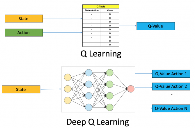
You may be wondering why we need to introduce deep learning to the Q-learning equation.
Q-learning works well when we have a relatively simple environment to solve, but when the number of states and actions we can take gets more complex we use deep learning as a function approximator.
Let's look at how the equation changes with deep Q-learning.
Recall the equation for temporal difference:
\[TD(a, s) = R(s, a) + \gamma max_{a'}Q(s', a') - Q_{t-1}(s, a)\]
In the maze example, the neural network will predict 4 values: up, right, left, or down.
We then take these 4 values and compare it to the values that were previously predicted, which are stored in memory.
So we're comparing $Q_1$ vs. $Q-Target1$, $Q_2$ vs. $Q-Target2$, etc.
Recall that neural networks work by updating their weights, so we need to adapt our temporal difference equation to leverage this.
So what we're going to do is calculate a loss by taking the sum of the squared differences of the Q-values and their targets:
\[L = \sum (Q-Target - Q)^2\]
We then take this loss and use backpropagation, or stochastic gradient descent, and pass it through the network and update the weights.
This is the learning part, now let's move on to how the agent selects the best action to take.
To choose which action is the best, we use the Q-values that we have and pass them through a softmax function.
This process happens every time the agent is in a new state.
7. Experience Replay
Now that we've discussed how to apply neural networks to Q-learning, let's review another important concept in deep Q-learning: experience replay.
One thing that can lead to our agent misunderstanding the environment is consecutive interdependent states that are very similar.
For example, if we're teaching a self-driving car how to drive, and the first part of the road is just a straight line, the agent might not learn how to deal with any curves in the road.
This is where experience replay comes in.
From our self-driving car example, what happens with experience replay is that the initial experiences of driving in a straight line don't get put through the neural network right away.
Instead, these experiences are saved into memory by the agent.
Once the agent reaches a certain threshold then we tell the agent to learn from it.
So the agent is now learning from a batch of experiences. From these experiences, the agent randomly selects a uniformly distributed sample from this batch and learns from that.
Each experience is characterized by that state it was in, the action it took, the state it ended up in, and the reward it received.
By randomly sampling from the experiences, this breaks the bias that may have come from the sequential nature of a particular environment, for example driving in a straight line.
If you want to learn more about experience replay, check out this paper from DeepMind called Prioritized Experience Replay.
8. Action Selection Policies
Now that we understand how deep Q-learning uses experience replay to learn from a batch of experiences stored in memory, let's finish off with how the agent actually selects an action.
So the question is: once we have the Q-values, how do decide which one to use?
Recall that in simple Q-learning we just choose the action with the highest Q-value.
As we mentioned earlier, with deep Q-learning we pass the Q-values through a softmax function.
In reality, the action selection policy doesn't need to be softmax, there are others that could be used, and a few of the most common include:
- $\epsilon$ greedy
- $\epsilon$-soft
- Softmax
The reason that we don't just use the highest Q-value comes down to an important concept in reinforcement learning: the exploration vs. exploitation dilemma.
To summarize this concept, an agent must make a tradeoff between taking advantage of what it already knows about the environment, or exploring further.
If it takes advantage of what it already knows it could gain more rewards, but if it doesn't explore further it may not be choosing the optimal actions.
9.Summary: Deep Q Learning
In this article, we looked at an important algorithm in reinforcement learning: Q-learning. We then took this information a step further and applied deep learning to the equation to give us deep Q-learning.
We saw that with deep Q-learning we take advantage of experience replay, which is when an agent learns from a batch of experience. In particular, the agent randomly selects a uniformly distributed sample from this batch and learns from this.
Finally, we looked at several action selection policies, which are used to tackle the exploration-exploitation dilemma in reinforcement learning.


