

In reinforcement learning, two of the main tasks of an agent include policy evaluation and control.
Policy evaluation refers to determining the value function for a specific policy, whereas control refers to the task of finding a policy that maximizes reward.
In other words, control is the ultimate goal of reinforcement learning and policy evaluation is usually a necessary step to get there.
In this article, we'll review a collection of algorithms called dynamic programming for solving the tasks of policy evaluation and control.
This article is based on notes from Week 4 of this course on the Fundamentals of Reinforcement Learning and is organized as follows:
- Dynamic Programming Algorithms
- Iterative Policy Evaluation
- Policy Improvement
- Policy Iteration
- Generalized Policy Iteration
- Efficiency of Dynamic Programming
Stay up to date with AI
Dynamic Programming Algorithms
Dynamic programming makes use of the Bellman equations discussed in our previous article to define iterative algorithms for both policy evaluation and control.
Before we review the algorithms, let's clearly define these two tasks.
Defining Policy Evaluation
Policy evaluation is the task of determining the state-value function $v_\pi$ for a given policy $\pi$
$$\pi \rightarrow v_\pi$$
Recall that the value of a state under a policy $v_\pi$ is the expected return from that state if the agent acts according to $\pi$
$$v_\pi(s) \doteq \mathbb{E}_\pi [G_t|S_t = s]$$
The return is the discounted sum of future rewards:
$$v_\pi (s) \doteq \mathbb{E}_\pi [R_{t+1} + \gamma G_{t+1} |S_t = s]$$
Also recall that the Bellman equation reduces the problem of finding $v_\pi$ to a system of linear equations for each state:
$$ = \sum\limits_a \pi(a|s) \sum\limits_{s'} \sum_r p(s', r | s, a)[r + \gamma v_\pi s']$$
In practice, however, solving for $v_\pi$ with the iterative practice of dynamic programming are more suitable than linear equations for general MDPs.
Defining Control
Control is the task of improving a policy.
The goal of the control task is thus to modify a policy to produce a new one which is strictly better.
In other words, if we have $\pi_1$ and $\pi_2$, the goal is to modify them create a new $\pi_3$ that has a value greater than or equal to the values of $\pi_1, \pi_2$ in every state.
We can iteratively try new policies to try and find a sequence of better and better policies over time.
When we can't improve the policy any further, the current policy must equal the optimal policy $\pi_*$, and the task of control is complete.
Below, we'll discuss how we can use the dynamics of the environment $\pi, p, \gamma$ to solve the tasks of policy evaluation and control.
Specially, we'll look at a class dynamic programming algorithms for this purpose.
Keep in mind that classical dynamic programming doesn't use interaction with the environment. Instead, it uses dynamic programming methods to compute value functions and optimal policies given a model $p$ of the MDP.
As we'll discuss, most reinforcement learnings are an approximation of dynamic programming without the model $p$.
In summary, dynamic programming algorithms can be used to solve both the tasks of policy evaluation and control, given that we have access to the dynamics function $p$.
Iterative Policy Evaluation
Dynamic programming algorithms work by turning the Bellman equations into iterative update rules.
In this section, we'll look at one dynamic programming algorithm called iterative policy evaluation.
Recall that the Bellman equation provides a recursive equation for the state-value of a given policy $v_\pi$:
$$ v_\pi = \sum\limits_a \pi(a|s) \sum\limits_{s'} \sum_r p(s', r | s, a)[r + \gamma v_\pi s']$$
Iterative policy evaluation takes the Bellman equation and directly uses it as an update rule:
$$v_{k+1}(s) \leftarrow \sum\limits_a \pi(a|s) \sum\limits_{s'} \sum_r p(s', r | s, a)[r + \gamma v_k s']$$
Now instead of giving us the true value function, we have a procedure to iteratively refine the estimate of the value function.
Ultimately, this process produces a sequence of better and better approximations of the value function over time.
As soon as the update rule leaves the value function unchanged, or when $v_{k+1} = v_k$ for all states, this means we've that found the value function $v_k = v_\pi$.
The only way that the update can leave $v_k$ unchanged is if it obeys the Bellman equation.
It can also be proven that for any choice of $v_0$, $v_k$ will converge to $v_\pi$ in the limit as $k$ approaches infinity:
$$\lim\limits_{k \rightarrow \infty} v_k = v_\pi$$
Implementing iterative policy evaluation involves storing two arrays, each of which has one entry for every state:
- One array is labeled $V$ and stores the current approximate value function
- The other array $V'$ stores the updated values
Using these two arrays allow you to compute the new values from the old one state at a time without changing the old values in the process.
At the end of each iteration, we can write all the new values $V'$ into $V$ and move on the the next iteration.
You can also implement a single array version of iterative policy evaluation, in which some updates use new values instead of old.
The single array version is still guaranteed to converge, and may in fact converge faster as it's able to use the updated values sooner.
To summarize, iterative policy evaluation allows you to turn the Bellman equation into an update rule that iteratively computes value functions.
Next, we'll look at how these concepts can be used for policy improvement.
Policy Improvement
In this section, we'll discuss the policy improvement theorem and how it can be used construct and improve policies.
We'll also look at how we can use the value function to produce a better policy for a given MDP.
Earlier we saw that given $v*$ we can find the optimal policy by choosing the greedy action $\underset{a}{\arg\max}$, which maximizes the Bellman optimality equation in each state:
$$\pi_*(s) = \underset{a}{\arg\max}\sum\limits_{s'}\sum\limits_r p(s', r, |s, a) [r + \gamma v_*(s')]$$
If instead of the optimal value function we select a greedy action with respect to the value function $v_\pi$ of an arbitrary policy $\pi$:
$$\pi_*(s) = \underset{a}{\arg\max}\sum\limits_{s'}\sum\limits_r p(s', r, |s, a) [r + \gamma v_\pi(s')]$$
We can then say that this new policy must be different than $\pi$, which is another way of saying that $v_pi$ obeys the Bellman optimality equation.
This means the new policy must be a strict improvement over $\pi$ unless $\pi$ is already optimal.
This is a result of a general rule called the policy improvement theorem, which states:
$$q_\pi (s, \pi'(s)) \geq q_\pi (s, \pi (s)) \:\text{for all}\: s \in \mathcal{S}$$
$q_\pi$ tells you the value of a state if you take action $A$ and follow policy $\pi$
The policy improvement theorem formalizes the idea that policy $\pi'$ is at least as good as $\pi$ if in each state the value of the action selected by $\pi'$ is greater than or equal to the value of action selected by $\pi$:
$$\pi' \geq \pi$$
Policy $\pi'$ is strictly better if the value is strictly great in at least one state.
In summary, the policy improvement theorem tells us that a gredified policy is a strict improvement unless the policy was already optimal. We also saw how to use a vlaue function udner a given policy to produce a strictly better policy.
Next, we'll look at how we can use this to create an iterative dynamic programming algorithm to find the optimal policy.
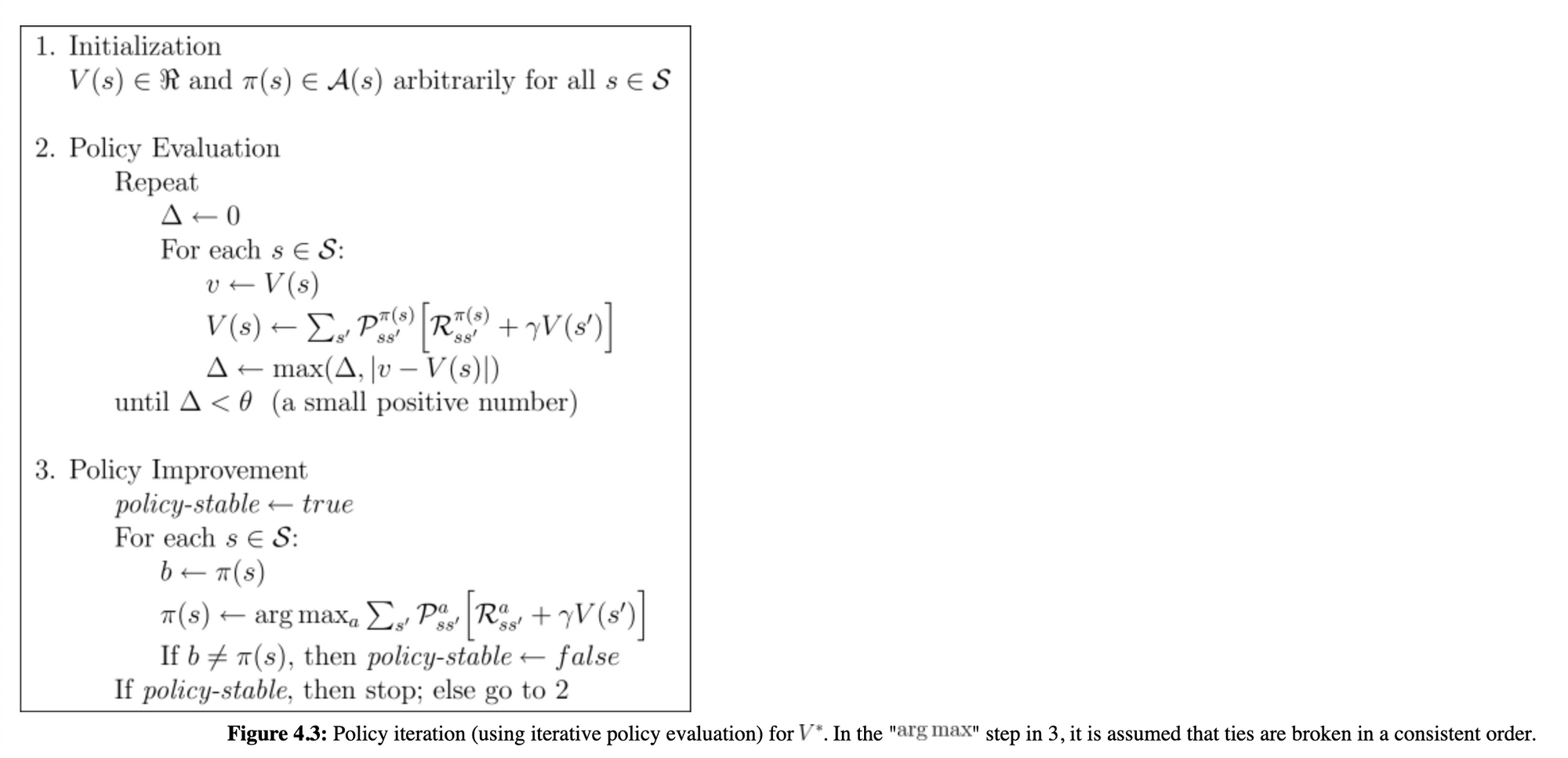
Policy Iteration
In this section we'll outline the policy iteration algorithm for finding the optimal policy, including:
- How policy iteration reaches the optimal policy by alternating between a evaluating a policy and improving it.
- How to apply policy iteration to compute optimal policy and optimal value functions
Recall that the policy improvement theoram says that unless the policy $\pi$ is optimal, we can construct a stricly better policy $\pi'$ than policy $\pi$ by acting greedily with respect to the value function of a given policy.
If we start with $\pi_1$, we can evaluate it using iterative policy evaluation to determine the state value $v_pi_1$. This is the evaluation step.
Using the policy improvement theorem, we can act greedily with respect to $v_pi_1$ to obtain a better policy $\pi_2$. This is the improvement step.
We can continue this process and compute $v_{\pi_2}$, improve on it to find $\pi_3$, and so on.
With this process, each policy is guaranteed to be an improvement unless the policy is optimal $\pi_*$, at which point we terminate the algorithm.
In this case, there are a finite number of deterministic policies, which means that it must eventually reach the optimal policy.
This process is referred to as policy iteration.
Policy iteration consists of alternating between evaluation and improvement over and over again until the optimal policy and optimal value function is reached.
Below is the policy iteration algorithm in pseudo-code from Sutton and Barto's book Reinforcement Learning: An Introduction:
Generalized Policy Iteration
We just discussed a strict policy iteration procedure of alternating between evaluating and improving the policy.
The framework of generalized policy iteration allows much more freedom while still guaranteeing an optimal policy.
The term generalized policy iteration refers to all alternative ways we can iteratively improve policy evaluation and policy improvement.
Value Iteration
One policy iteration algorithm is called value iteration.
In value iteration we sweep through all the states and greedify them with respect to the current value function, although we don't run policy evaluation to completion.
Instead, we just perform one sweep through all states and then we greedify again.
Below is the algorithm for value iteration from Reinforcement Learning: An Introduction:
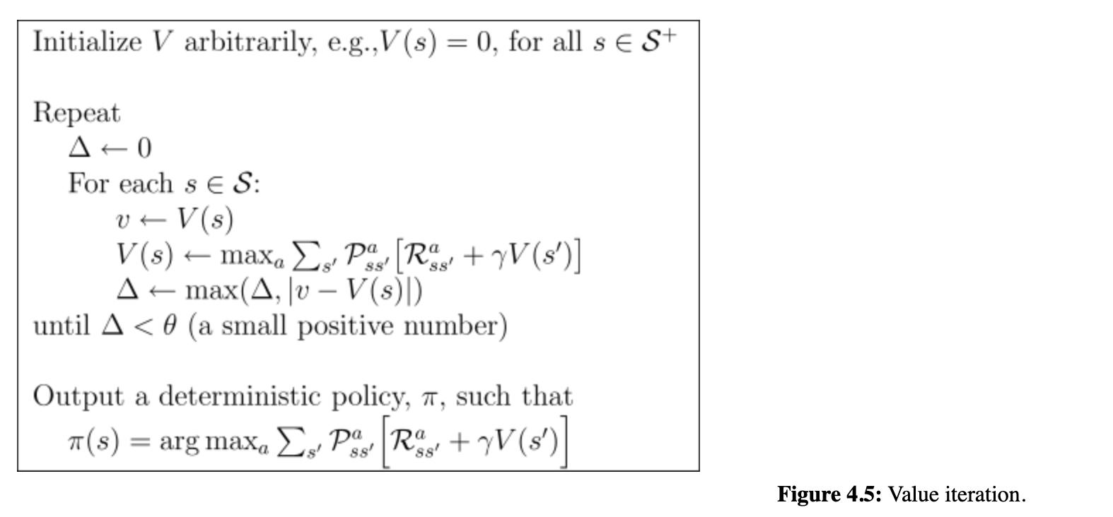
This is similar to iterative policy evaluation, although instead of update the value to a fixed policy we update use the action that maximizes the current value estimate.
In summary, value iteration allows us to combine policy evaluation and improvement into a single update.
Efficiency of Dynamic Programming
In this section, we'll discuss Monte Carlo Sampling as an alternative method for learning a value function.
We'll also describe the Brute-Force Search as an alternative to finding an optimal policy.
To conclude, we'll review the advantages of dynamic programming over these alternatives.
Monte Carlo Sampling
One alternative method for learning the value function is with Monte Carlo Sampling.
Recall that the value is the expected return from a given state.
In this method we gather a large number of returns under $\pi$ and take their average, which will eventually converge to the state value.
This issue with this method is that we may need a large number of returns from each state.
Since each return depends on many actions selected by $\pi$ and many state transitions, we may be dealing with a lot of random information with this approach.
This would require average many returns before the estimate converges.
A key insight of dynamic programming is that don';t have to treat each state evaluation as a separate problem.
Instead, by using the value estimates of future states allows us to compute the current value estimate more efficiently. This process is known as bootstrapping.
Brute Force Search
Brute force search refers to evaluating every possible deterministic policy one at a time and then choosing the policy with the highest value.
The issue, however, is that the total number of deterministic policies is exponential with the number of states.
This means that with even relatively simple problems the number of policies can be massive.
Since the policy improvement theorem finds a better and better policy with each step, this is a significant improvement over brute force search.
The efficiency of dynamic programming can be summarized as follows:
Policy iteration is guaranteed to find the optimal policy in polynomial time in the number of states $|\mathcal{S}|$ and actions $|\mathscr{A}|$.
In general, solving an MDP gets exponentially harder as the number of states grows. This makes dynamic programming exponentially faster than a brute force search.
Summary: Dynamic Programming
Dynamic programming can be used in reinforcement learning to solve the tasks of policy evaluation and control.
Policy evaluation is the task of determining the state-value function $v_\pi$ for a given policy $\pi$.
Iterative policy evaluation uses the Bellman equation for $v_\pi$ and turns it into an update rule, which produces a sequence of better and better approximations.
Control is the task of improving a policy.
The policy improvement theorem provides a framework for constructing a better policy from a given policy.
With this theorem, $\pi'$ is guaranteed to be better than $\pi$ unless it was already optimal.
The policy iteration algorithm relies on this theorem and consists of alternating between policy evaluation and improvement. These steps are repeated until the policy doesn't change is thus optimal.
In generalized policy iteration, the steps of policy evaluation and improvement do not need to run until completion, which can be particularly useful if we have a large state space.
In summary, the concepts of dynamic programming are fundamental to many reinforcement learning algorithms in use today.


