
In this guide in our Mathematics of Machine Learning series we're going to cover an important topic: multivariate calculus.
Before we get into multivariate calculus, let's first review why it's important in machine learning.
Calculus is important because in order to optimize a neural network, we use variations of gradient descent, the most common of which is stochastic gradient descent.

This article is based on this Mathematical Foundation for Machine Learning and AI, and is organized as follows:
- Introduction to Derivatives
- Introduction to Integration
- Introduction to Gradients
- Gradient Visualization
- Mathematical Optimization
Stay up to date with AI
1. Introduction to Derivatives
The definition of a derivative can be understood in two different ways.
The first way is in a geometric perspective, where the derivative is the slope of a curve. Essentially it is how much a curve is changing at a particular point.
The second is a physical perspective, where the derivative is the rate of change.
As we can see both of these perspectives are related to change.
Derivative Notation
The derivative operator is written as:
\[\frac{d}{dx}\]
This could read as the derivative with respect to $x$.
Scalar Derivative Rules
This is not an exhaustive list of the rules, but let's review a few of the basics.
Constants - the derivative of any constant is 0.
\[\frac{d}{dx}c = 0\]
For example:
\[\frac{d}{dx}55 = 0\]
This makes sense when you think about change, because the constant 55 is not changing at all.
Power Rule - this is how you deal with variables in derivatives. If we have a derivative of $x^n$ with respect to $x$, we calculate this as follows:
\[\frac{d}{dx}x^n = nx^{n-1}\]
For example:
\[\frac{d}{dx}x^4 = 4x^3\]
Multiplication - this is how we deal with multiplication of derivatives:
\[\frac{d}{dx}cx^n = c\frac{d}{dx}x^n = cnx^{n-1}\]
The Sum Rule - if we have two functions and they are added together we can take the derivative of them both indivually:
\[\frac{d}{dx}(f(x) + g(x)) = \frac{d}{dx}f(x) + \frac{d}{dx}g(x)\]
The Product Rule - multiplying two functions together is a bit more complicated, we take the derivate of the first function times the second plus the derivative of the second times the first:
\[\frac{d}{dx}(f(x)g(x)) = g(x)\frac{d}{dx}f(x) + f(x)\frac{d}{dx}d(x)\]
The Chain Rule - the chain rule is important for machine learning because when we have multiple layers in a neural network we need this calculate the derivative of earlier layers. If we have a function $g(x)$ inside another function $f(x)$, we take the derivative of the outside function $f'$ times the derivative of the inside function $g'$:
\[\frac{d}{dx}(f(g(x)) = f'(g(x))g'(x))\]
These are just a few important rules, but let's move on to partial derivatives.
Partial Derivatives
Partial derivatives are used for equations with more than one variable.
If we have two variables we have the partial with respect to $x$ and the partial with respect to $y$:
\[\frac{d}{dx} \frac{d}{dy}\]
Now let's move on to integrals, which are essential to probability theory.
2. Introduction to Integration
Let's now discuss integrals in the context of machine learning.
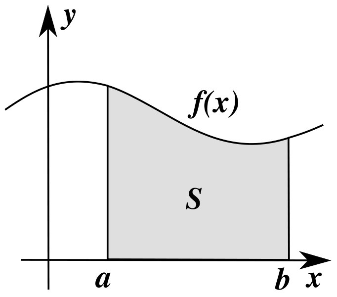
Integration is used to find the area under a curve. The integral is the opposite of differentiation, and is often referred to as the anti-derivative.
There are two types of integrals: definite and indefinite.
Definite integrals have limits, and can be written as follows:
\[\int_a^b f(x)dx\]
Indefinite integrals have no limits, so we're taking the integral from negative infinity to positive infinity:
\[\int f(x)dx\]
As mentioned, the integral can be understood as the anti-derivative as it reverses differentiation.
In the equation below we have the integral of $f'(x)$ is equal to $f(x)$, so if we take the integral of a function we get back the original function.
\[\int f'(x)dx = f(x) + C\]
The $C$ term is referred to as the constant of integration and is there because the derivative of a constant is 0, so we don't know if it was there or not.
The Rules of Integration
Let's review a few of the rules of integration.
The Power Rule - this is the reverse of the power rule in derivatives:
\[\int x^n dx = \frac{x^{n+1}}{n+1} + C \]
Constants - these follow the power rule:
\[\int kdx = kx + C\]
Evaluating Definite Integrals
If we have limits on our integral $a$ and $b$ we evaluate them as follows:
\[\int_a^b f(x)dx\]
This is the same as saying the (value of $f(x)$ + $C$ at $x=b$) - (value of $f(x)$ + $C$ at $x=a$). Since the $C$'s are going to cancel out we're left with:
\[\int_a^b f(x)dx = f(b) - f(a)\]
This can also be written as:
\[\int_a^b f(x)dx = f(x)|_a^b = f(b) - f(a)\]
We'll discuss integrals more in our article on probability theory, but let's now move on to the concept of gradients.
3. Introduction to Gradients
Gradients are extremely important in machine learning because this is how we optimize neural networks.
To understand gradients we need to return to partial derivatives, which we can reorganize into a vector as shown below:
\[\frac{d}{dx} and \frac{d}{dy}\]
\[\nabla = \vec{\frac{d}{dx}, \frac{d}{dy}}\]
where $\nabla$ is the gradient.
Let's look at an example - if we have the gradient for $f(x, y)$ this is the same as writing the partial of $f$ with respect to $x$ and the partial with respect to $y$:
\[\nabla f(x,y) = \vec{\frac{df(x,y)}{dx}, \frac{df(x,y)}{dy}}\]
Understanding the Gradient
As you may have guessed, like the derivative, the gradient represents the slope of a function.
The gradient points in the direction of the largest rate of increase of the function, and its magnitude is the slope in that direction.
This is very valuable because we can determine the direction to change our variables that will have the greatest impact.
In the context of machine learning we take the negative gradient direction to minimize our loss function.
Gradient Vectors
It's important to note that gradients are not restricted to two dimensions like we've seen, and are often expanded into higher dimensions.
In the context of machine learning we rarely stop at 3 dimensions, so gradient vectors can be organized as partial derivatives for a scalar function. If there are multiple functions, we use the Jacobian, which is a vector of gradients.
Let's now look at convex optimization and see how we can use gradients to minimize the loss function in our machine learning algorithm.
5. Mathematical Optimization
We're now going to combine all of the multivariate calculus we've discussed and look at how they apply to the process of optimization.
Optimization is at the core of modern machine learning, specifically in regards to deep neural networks.
This is the process of how we get our learning algorithms to actually learn from data and update its own parameters.
The Optimization Problem
The optimization problem is often stated as follows - we want to minimize a function $f_0(x)$ subject to particular constraints:
minimize $f_0(x)$
s.t. $f_i(x) \leq 0, i = {1,...,k}$
$h_j(x) = 0, ij= {1,...,l}$
It is the objective function or $f_0$ that we're trying to minimize, and in machine learning this would be our loss function.
We also have an optimization variable $(x)$, which are the variables that go into our objective function. These are often the parameters we want to update iteratively.
The constraint functions can vary, and the example above is for a convex optimization function.
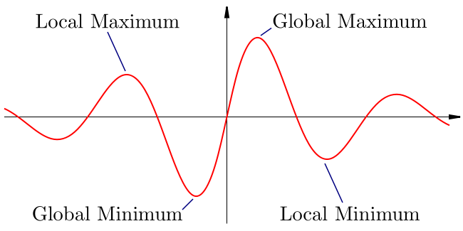
Optimization seeks to find the global minimum for an objective function, subject to constraints.
A global minimum is the lowest point on a graph, as shown in the image below, and the red line represents the objective function:
Local minimums are also important in machine learning because when we optimize our algorithms we can often get stuck in local minimums.
As mentioned, optimization is extremely important in machine learning because this is how they actually learn and improve through an iterative process of minimizing an objective function.
The steps to solve an optimization problem include:
- The the first derivative test of $f(x)$
- Use the second derivate test to prove that it is a minimum vs. a maximum
In the context of machine learning optimization is an iterative process, where we first guess and then take the gradient to tell us which way to change the parameters.
We do this over and over again until our guesses no longer improve the results, and how much we update the guess each time is referred to as the learning rate.
Summary: Multivariate Calculus for Machine Learning
Continuing in our Mathematics for Machine Learning series, in this article we introduced multivariate calculus.
As discussed, multivariate calculus is extremely important in machine learning because we use optimization in order to improve our neural network. In particular, we use variations of gradient descent to optimize a neural network.
To introduce this concept we first looked at derivatives, which refers to the rate of change of a particular function.
We then looked at integrals, which are used to find the area under a curve. The integral is often referred to as the anti-derivative as it is the opposite of differentiation.
Next we introduce gradients, which as mentioned are very important in optimizing a neural network. The gradient represents the slope of a function and points in the direction with the largest rate of increase.
The gradient is very valuable in machine learning because it allows us to minimize our loss function, and also determine the direction to change our variables that will have the greatest impact.
Finally we combined all of these concepts together and looked at how they apply to the process of optimization.
Optimization is the process by which machine learning algorithms actually learn from data and update their own parameters iteratively. In particular, we improve the performance of our model through an iterative process of minimizing an objective function, or the loss function.
We keep iterating through this process until it no longer improves the results.
That's it for this introduction to multivariate calculus, and of course we could cover each topic in much more depth, but for now we just want a high-level overview of how multivariate calculus applies to machine learning.
In the next article we'll look at probability theory, which is is another essential concept to the statistical learning used in the field of machine learning.