
In this article, we'll introduce fundamental concepts of quantitative modeling for finance. In particular, we'll review the quantitive modeling workflow, common vocabulary, and several mathematical functions. Finally, we'll look at a core building block of quantitive modeling: linear models.
This article is based on notes from this course on Fundamentals of Quantitive Modeling and is organized as follows:
- What is Quantitative Modeling?
- Key Steps in the Quantitative Modeling Process
- Quantitative Modeling Vocabulary
- Mathematical Functions for Quantitative Modeling
- Linear Models & Optimization
What is Quantitative Modeling?
First, we need to define what a model actually is.
A model is a formal description of a business process.
Models typically involve mathematical equations and/or random variables.
Models are almost always a simplification of a more complex structure or reality, making the modeling process both an art and science.
Models rely on a set of assumptions and are usually implemented using a computer program or spreadsheet.
Examples of Models
A few examples of models include:
- The price of a diamond as a function of weight, which could potentially be modeled with a linear function
- The relationship between demand and price of a product, which could be modeled with a power function to determine the optimal price
- The uptake of a new product in a market, which could be modeled with a logistic function
We'll discuss each of these functions in more detail later.
Examples of Modeling in Practice
A few examples of how models are used in practice include:
- Prediction: This involves calculating a single output.
- Forecasting: This involves predicting time-series data in the future.
- Optimization: An example of optimization is determining the price that will maximize profit.
- Ranking and targeting: This often involves limited resources and identifying targets for opportunity.
- What-if scenarios: Modeling can be use to predict potential outcomes of various scenarios.
- Sensitivity analysis: These are used in order to assess how sensitive a model is to its key assumptions.
After applying models to these use cases, a few examples of the potential benefits include:
- Identifying gaps in current understanding
- Making assumptions explicit
- Describing business processes accurately
- Using insights as a decision support tool
Stay up to date with AI
Key Steps in the Quantitative Modeling Process
Every model is different, although they typically share a common high-level workflow.
Below is an example of a 7 step modeling workflow:
- The modeling process workflow begins by identifying inputs and outputs.
- The next step is to define the scope of the model, or the intended use case of the model.
- Once you have the inputs, outputs, and score, the next step is to formulate the model using the mathematical techniques discussed below
- After formulating the model, you need to perform a sensitivity analysis to assess the models assumptions.
- The next step is to validate the models forecasts or predictions with real-world data
- Next, we need to determine if the model is fit for its intended purpose. This doesn't necessarily mean is the model is right, as models are a simplification of reality, but you need to determine if its within the defined scope.
- If the model is within the intended scope, it should then be implemented. If not, you'll need to return to defining the scope and formulating the model.
Keep in mind that modelling is a continuous and evolutionary process that almost always requires identifying weaknesses, limitations, and iteration in the modeling process to improve it.
Quantitative Modeling Vocabulary
Now that we've reviewed what modeling is and a high-level workflow, let's look at some common vocabulary.
Data Driven vs. Theory Driven Models
Quantitative models will often fit on a spectrum between empirical and theoretical.
A theoretical model says that given a set of assumptions and relationships, what are logical consequences?
An example of a theoretical assumption is that markets are efficient.
A data driven model says that given a set of observations, how can we approximate the underlying processes that generated them?
An example of a data driven model would be to split customer into profitable and unprofitable ones and try to model the features that differentiate them.
Deterministic vs. Probabilistic Models
A deterministic model means that given a set of fixed inputs, the model will always output the same answer.
A probabilistic model means that with identical inputs, the model's output can vary from instance to instance.
Discrete vs. Continuous Models
Discrete models are characterized by distinct values, for example integers, and are not infinitely divisible.
Continuous models are a smooth process with an infinite number of potential values in any fixed interval.
Static vs. Dynamic Models
Static models capture a single snapshot of a business process.
Dynamic models describes the evolution of the process over time. In other words, it describes the movement from state to state.
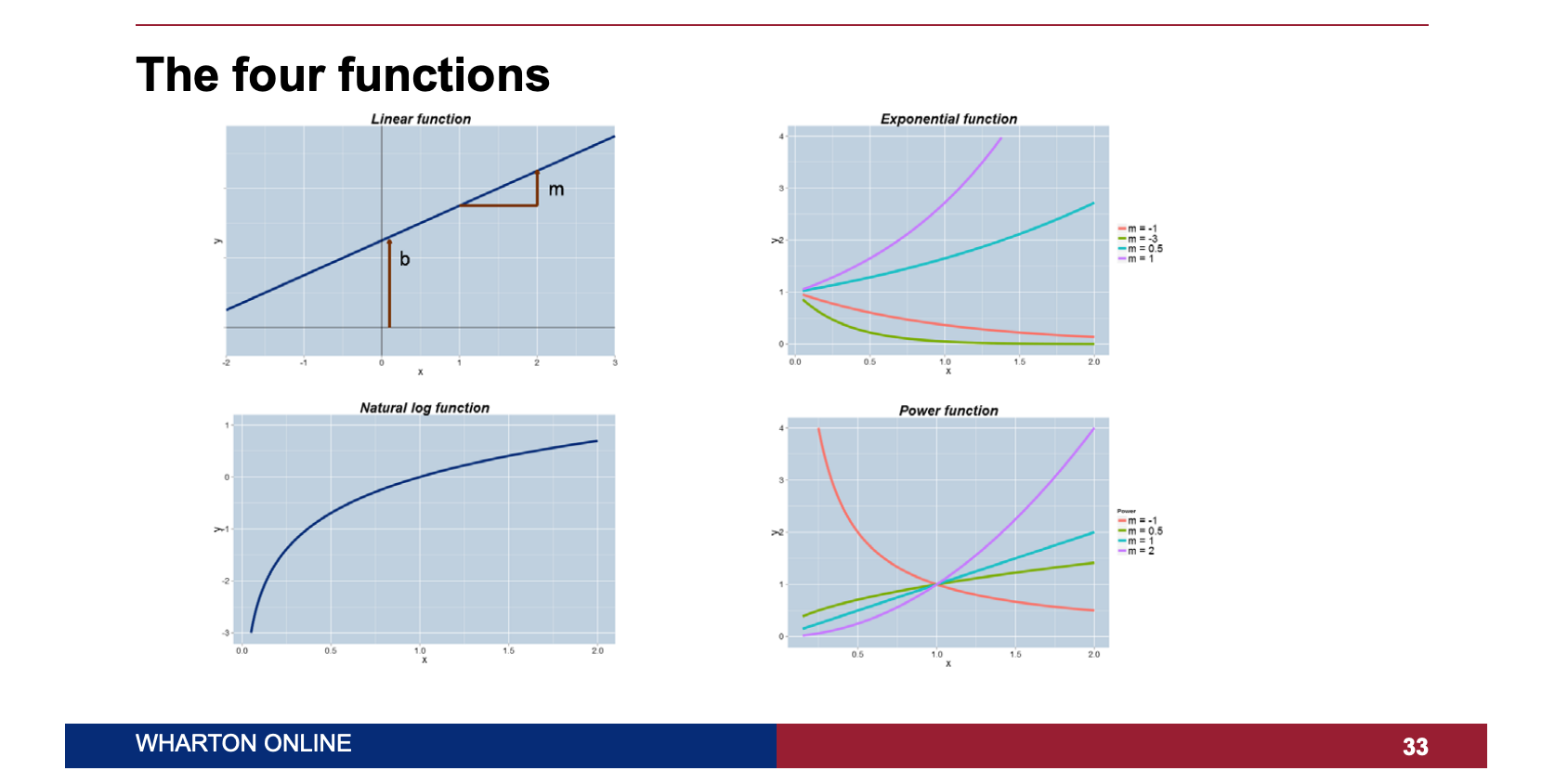
Mathematical Functions for Quantitative Modeling
In this section we'll look at four key mathematic functions used in quantitative modeling, including:
- Linear
- Power
- Exponential
- Logarithmic
Linear Functions
A linear function is a core building block of quantitative models.
Linear functions are characterized by the intercept $b$ and slope $m$. The equation for a linear function is $y = mx + b$, where:
- $x$ is the input to the model
- $y$ is the output of the model
- $b$ is the height of the line above the origin at the $x$ axis
- $m$ tells you how much $y$ has gone up as $x$ moves by one unit
As essential characteristic of linear models is that the slope is constant.
Power Functions
A power function is written as $y = x^m$.
Examples you may be familiar with include:
- $m=1$ we get a linear function
- $m=2$ we get a quadratic
- $m=0.5$ we get a square root
The essential characteristic of a power function is that if $x$ changes by one percent, $y% will change by approximately $m$ percent.
Below are a few more examples of power functions:
Exponential Functions
To form an exponential function, the independent variable is an exponent.
Exponential functions can be written as $y = e^{mx}$, where:
- $e$ is the mathematical constant 2.71828...
The essential characteristic of exponential functions is that the rate of change of $y$ is proportional to $y$ itself.
Logarithmic Functions
The log function is one the most commonly used transformations in quantitative modeling.
A log function is written as $y = log_b(x)$, where:
- $b$ is the base of the logarithm
- The most frequently used base is the number $e$ and the logarithm is called the "natural log"
A log curve is an increasing function, although it's increasing at a decreasing rate. A log function is very useful for modeling processes that exhibit diminishing returns to scale.
An essential characteristic of log functions is that a proportionate change in $x$ is associated with the same absolute change in $y$.
Below is a visualization of each of these four functions from Week 1 of this course on Quantitative Modeling:
Linear Models and Optimization
In this section we'll look at linear models in more detail, in particular:
- Linear cost functions
- Linear programming
- Growth and decay in discrete time
- Present and future value
- Continuous compounding
- Classical optimization
Recall that linear functions have a constant slope. In practice, it's useful to ask yourself if a constant slope assumption is realistic, and if not, a linear model may not be appropriate.
Linear Cost Function
An example of a linear model is a linear cost function.
In this example we'll call the number of units produced $q$ and the cost of producing $q$ units $C$. The linear equation of this cost function is $C = 100 + 30q$.
The two coefficients can be interpreted as follows:
- $b$ is the total cost of producing 0 units, or the part of the total cost that doesn't depend on the quantity produced. In other words, it's the fixed cost.
- $m$ is the slope of the line and is the change in total cost of an incremental unit of production, or the variable cost.
Linear Programming
One of the key uses of linear models is in linear programming (LP), which is a technique to solve certain optimization problems.
These models incorporate constraints to make them more realistic.
These linear programming problems can typically be implemented with add-ons in common spreadsheets.
Growth and Decay in Discrete Time
Growth is a fundamental concept in business and finance, and a linear model may sometimes be appropriate for a growth process.
An alternative to a linear (additive) growth model is proportionate growth, in which there's a constant percent increase or decrease from one period to the next.
Constant proportionate growth is called a geometric progression or geometric series.
Present and Future Value
A key application of these growth models are in the calculation of present and future value.
Present value is the expected current value of an income stream and is calculated as follows:
$$P_t = P_0\theta^t$$
where,
- $\theta$ is the constant proportional growth factor
Use cases of present value include discounting investments to the present time. For example, an annuity is a schedule of fixed payments over a period of time. The present value of annuity is the sum of the present values of each separate payment
Continuous Compounding
The compounding of an investment can be yearly, monthly, weekly, daily, etc.
As the compounding period gets shorter and shorter, the process is said to be continuously compounded.
Mathematically, if we have a principal amount $P_0$ that is continuously compounded at a nominal annual interest rate of $R$%, then at year $t$ $P_t = P_0e^{rt}$ where $r = R/100$
In a continuous model, the value $t$ can take on any value in an interval, whereas the discrete model $t$ can only take on distinct values.
Optimization
To conclude this section on linear models, we'll look at an optimization problem, which is classical in the sense that it's solve using calculus.
A common modeling objective is to perform a subsequent optimization.
The objective of the optimization is to find the value of an input that either maximizes or minimizes and input. For example, you can use optimization to determine the price that maximizes profit.
To solve an optimization problem using calculus involves the technique of differentiation. In particular, we need to find the derivative, or the rate of change, of profit with respect to price equaling 0.
With calculus, we can obtain an optimal value of price as:
$$p_{opt} = \frac{c b}{1 +b'}$$
where
- $c$ is the production cost and $b$ is the exponent in the power function
The value of $-b$ is known as the price elasticity of demand.
Summary: Quantitative Modeling for Finance
As discussed in this introduction to quantitive modeling, a model is a formal description of a business process. Models are almost always simplifications of more complex structures, which make the process both an art and a science.
Examples of models in practice include prediction, forecasting, optimization, ranking, what-if scenarios, and sensitivity analyses.
Next, we discussed essential vocabulary for quantitive modeling, including
- Data-driven vs. theory driven models
- Deterministic vs. probabilistic models
- Discrete vs. continuous models
- Static vs. dynamic models
We then looked at common mathematical functions used in modeling, including linear functions, power functions, exponential functions, and logarithmic functions. Finally, we concluded by looking at linear models and optimization in more detail.
In the next article, we'll discuss an essential skill in quantitative modeling for finance: probabilistic models.