Introduction to Quantum Programming with Qiskit

In this guide we're going to look at quantum programming with Qiskit: the Quantum Information Science Kit. Released in 2017 and founded by IBM Research, Qiskit is:

An open-source quantum computing framework for leveraging today's quantum processors in research, education, and business

In this guide we'll assume you have some knowledge of quantum mechanics and quantum computation, but if you don't check out these articles on the subject:

• Quantum Machine Learning: Introduction to Quantum Systems
• Quantum Machine Learning: Introduction to Quantum Computation
• Quantum Machine Learning: Introduction to Quantum Learning Algorithms
• Introduction to Quantum Programming with Google Cirq
• Quantum Programming with the D-Wave Quantum Annealer

This guide is based on notes from this tutorial from Sentdex, and is organized as follows:

1. Getting Started with Quantum Programming
2. Qubits & Quantum Gates
3. Programming the Deutsch Jozsa Algorithm with Qiskit

1. Getting Started with Quantum Programming

While we won't go into the theoretical concepts behind quantum mechanics and quantum computation (like superposition and entanglement) in this article, let's very briefly review the practical concepts to get start with the programming side of things.

The first concept to understand is the difference between programming a classical bit vs. programming a qubit.

1.1 Classical Bits vs. Qubits

In a classical bit, the number of states you can represent with each bit is 2 - either a 0 or a 1, so the total number of states will be $n$ bits x 2.

In a quantum computer, a qubit can be 0, 1, or both states. When we have multiple qubits this makes the total number of states we can represent $2^n$ bits.

Since the quantum computer is exponential, this makes a massive difference in the number of states we can consider with each step of computation. While quantum computers won't completely replace classical computers, they're designed to solve the problems that classical computers simply can't solve in a reasonable timeframe.

1.2 Installing Qiskit & Importing Packages

We're going to make use of Google Colab for this tutorial, although you can also just create a new Qiskit notebook from within your IBM Q account. That said, let's first install the necessary packages to work with Qiskit.

!pip install qiskit
!pip install qiskit-ibmq-provider

Next we can import the necessary packages into our notebook:

import qiskit as q
%matplotlib inline

1.3 Defining Quantum Circuits

Next we have to build our quantum circuits, which actually work together with classical bits. For example, the following code will build a 2 qubit, 2 classical bit circuit:

# build a 2 qubit, 2 classical circuit
circuit = q.QuantumCircuit(2,2)

Then we're going to apply a NOT gate to the qubit, which makes it 10. We then apply a CNOT gate which will entangle the two qubits. What the CNOT gate does is it flips the 2nd qubit value if the first qubit is a 1. What we should get after this is a 11 state:

# apply a NOT gate to qubit 0, currently 0,0
circuit.x(0)
# now 10

# apply a CNOT gate, which flips 2nd qubit value if first qubit is a 1
circuit.cx(0, 1)
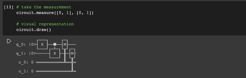
# now 11

We can then take the measurement, although it's important to note that by taking this measurement we do collapse any qubits that were in superposition. We take the measurement by specifying the qubit register (how it will map to the classical bit). So what we should get here is 11 (represented as classical bits):

# take the measurement
circuit.measure([0, 1], [0, 1])

We can also get a visual representation of our circuit with the circuit.draw() method:

1.4 Running Circuits on the IBM Quantum Computer

In order to run this circuit on the IBM quantum computer, you will need to get your token from the "My Account" section of IBM Q.

from qiskit import IBMQ

IBMQ.save_account("YOUR TOKEN")

You only need to do this once, and then you can use IBMQ.load_account() to load your account.

There are several backends that we can send our request to at IBM Q, including:

• ibmq_qasm_simulator
• ibmq_16_melbourne
• ibmq_ourense
• ibmqx2
• ibmq_vigo
• ibmq_london
• ibmq_burlington
• ibmq_essex
• ibmq_armonk

Before we specify which backend we want to use we can take a look at the queue and the number of qubits of each backend:

# choose backend
provider = IBMQ.get_provider("ibm-q")

for backend in provider.backends():
  try:
    qubit_count = len(backend.properties().qubits)
  except:
    qubit_count = "simulated"

  print(f"{backend.name()} has {backend.status().pending_jobs} queued and {qubit_count} qubits")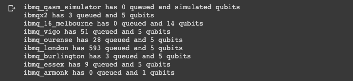

Let's go with imbqx2 since the queue isn't that long and has enough qubits for our job. Now we can choose that backend to run our circuit, and we can specify the number of shots, which is how number of repetitions of each circuit, to make sure we get an adequate representation:

from qiskit.tools.monitor import job_monitor

backend = provider.get_backend("imbqx2")
job = q.execute(circuit, backend=backend, shots=500)
job_monitor(job)

We can now visualize our result with the following code:

from qiskit.visualization import plot_histogram

result = job.result()
counts = result.get_counts(circuit)

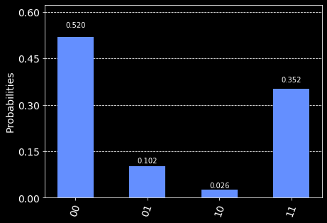
plot_histogram([counts])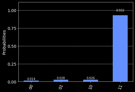

From this graph we can see the 11 had the highest probability (which is correct), but we can also see that the other options had a small probability. The reason for this is due to quantum noise, which refers to the "uncertainty of a physical quantity that is due to its quantum origin".

Now that we've looked at an example of entanglement with the CNOT gate, let's change our circuit slightly and look at a Hadamard gate, which puts the qubit in superposition.

# definfe the backend
backend = provider.get_backend("ibmq_burlington")

# qubits, 2 classical bits
circuit = q.QuantumCircuit(2, 2)

# apply a hadamard gate, which puts the qubit in superposition
circuit.h(0)

# apply a CNOT gate, which flips 2nd qubit value if first qubit is a 1
circuit.cx(0, 1)

# take the measurement
circuit.measure([0, 1], [0, 1])

# draw the circuit
circuit.draw()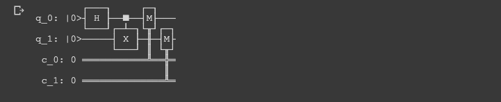

Now if we run our job again with the ibmq_burlington backend we get the following result:

Here we can see that there is still some quantum noise, but the highest probabilities are assigned to 00 and 11 since the qubits are superimposed.

2. Qubits & Quantum Gates

Now that we've look at running 2 basic circuits on IBM Q, let's review what's actually happening to the qubits and gates.

To do this we'll visualize qubits on the Bloch sphere, which is:

a geometrical representation of the pure state space of a two-level quantum mechanical system (qubit)

We won't get into detail about the Bloch sphere here, but as you can see from the image below you've got the $|0\rangle$ state at the top of the sphere and $|1\rangle$ at the bottom of the sphere.

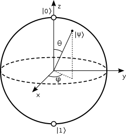
From the middle of the sphere we have the qubits actual vector, which could be pointing to 0 or 1, but it also be pointing anywhere else in the sphere. When we take our measurement we get back a probability of states.

Before we take our measurement, we can apply our gates to it, which take our vector and apply some form of rotation to it. And as we'll see, we can visualize the qubits at the output stage with Qiskit.

2.1 Visualizing Qubits on the Bloch Sphere

We're just going apply a few gates to circuits and visualize the result on the Bloch sphere, but you can find the entire list of gates that you can apply to a quantum circuit here.

Earlier we looked at the CNOT gate for entanglement, the Hadamard gate for superposition, and the rest of the gates apply some form of rotation.

First we want to import several visualization modules from Qiskit:

from qiskit.tools.visualization import plot_bloch_multivector
from qiskit.visualization import plot_histogram

Next we're going to use the statevector simulator from Qiskit Aer to plot the Bloch vector and then the qasm_simulator to get the probability distribution outputs:

statevector_sim = q.Aer.get_backend("statevector_simulator")
qasm_sim = q.Aer.get_backend("qasm_simulator")

Now we're going to write a function to run our job so we can visualize the changes along the way:

def run_job(circuit):
  result = q.execute(circuit, backend=statevector_sim).result()
  statevec = result.get_statevector()

  n_qubits = circuit.n_qubits
  circuit.measure([i for i in range(n_qubits)], [i for i in range(n_qubits)])

  qasm_job = q.execute(circuit, backend=qasm_sim, shots=1024).result()
  counts = qasm_job.get_counts()
  return statevec, counts

Now let's create a basic 2 qubit, 2 classical bit circuit and visualize the state vector:

circuit = q.QuantumCircuit(2,2)
statevec, counts = run_job(circuit)
plot_bloch_multivector(statevector)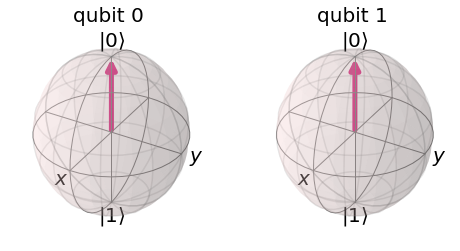

Here we can see that the measurement will always collapse the qubit to (0,0).

Let's now put qubit 1 into superposition with a Hadamard, so now the output could be a 0 or a 1.

circuit = q.QuantumCircuit(2,2)

# put qubit 1 in superposition
circuit.h(1)

statevec, counts = run_job(circuit)
plot_bloch_multivector(statevector)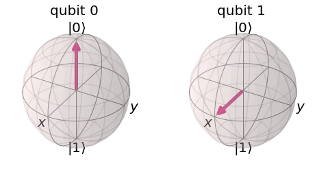

From this we can see that the Hadamard gate rotated the vector along the $y$ axis.

Now let's look at what happens if apply a Hadamard gate to qubit 0 and a CNOT gate to qubit 1:

# put qubit 0 in superposition & CNOT on qubit 1
circuit.h(0)
circuit.cx(0,1)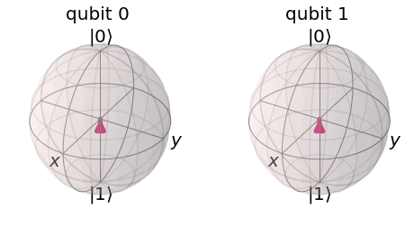

Here we can see the CNOT gate after the Hadamard gate changes qubits go to this centered state. Since they are now entangled from the CNOT gate, instead of getting four combinations of output (00, 01, 10, 11) we only get two possibilities (00 and 11):

plot_histogram([counts])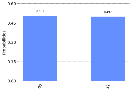

3. Programming the Deutsch Jozsa Algorithm with Qiskit

Now that we've visualized what's happening to the qubits as we apply gates to them on the Bloch sphere, let's look at an example of an algorithm that shows how quantum computer can outperform a classical computer.

3.1 What is the Deutsch Jozsa algorithm?

The Deutsch Jozsa algorithm is a good place to start since it was the first example of a quantum algorithm that performs better than the best classical algorithm.

It is not necessarily the result of the algorithm that is important here, but seeing how a quantum circuit can consider all the possible inputs and can immediately respond with an output.

If you want to learn more details about the Deutsch Jozsa algorithm check out the Qiskit documentation on it, but here is a summary:

• We have a hidden Boolean function which takes as input strings of bits and returns either 0 or 1
• The question we want answered is if the output will be a constant output, meaning all 0's or all 1's, or a balanced output, meaning an even number of 0's and 1's
• On a classical computer, if we had a 2 bit string it would take a least 2 queries in order to figure out if it is constant or balanced. As we increase the number of bits that we want to pass through this function it will take exponentially longer with each new bit
• A quantum circuit, on the other hand, can make this determination in 1 query, regardless of how long the bit string is

As you can see the problem that we're solving is not that useful, but this algorithm really demonstrates the unique attributes that quantum circuits have that their classical counterparts do not.

3.2 Defining the Quantum Circuit

Let's define the circuit to implement the Deutsch Jozsa algorithm in Qiskit. Here are the steps:

• Define a 2 qubit, 2 classical bit circuit
• Rotate on y with math.pi/4 on qubit 0
• Do the same thing on qubit 1
• Create the original state vector by executing the circuit on the statevector_simulator

c = q.QuantumCircuit(2,2)
c.ry(math.pi/4, 0)
c.ry(math.pi/4, 1)
orig_statevec = q.execute(c, backend=statevec_sim).result().get_statevector()
c.measure([0,1], [0,1])
c.draw()

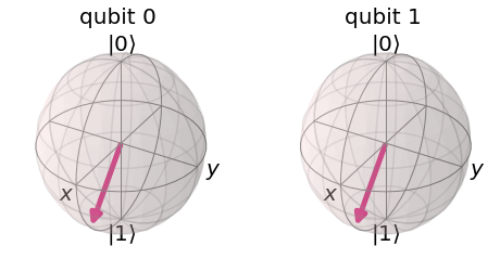
Now that we have our rotations and our measurements let's plot the original state vector on the Bloch sphere:

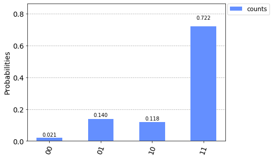
Now let's get the counts of the circuit with the qasm_simulator and plot the histogram:

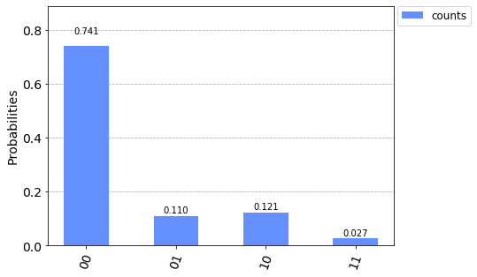
orig_counts = q.execute(c, backend=qasm_sim, shots=1024).result().get_counts()
plot_histogram([orig_counts], legend=['counts'])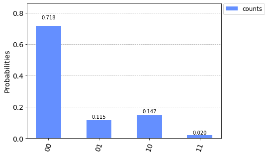

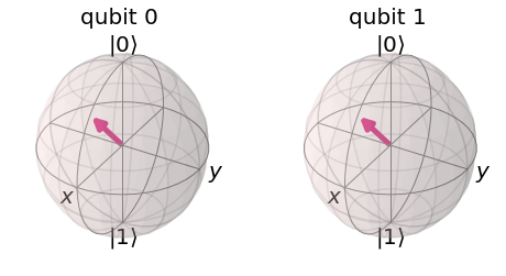
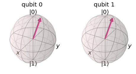
So far we have defined uncertain qubits, and now we're going to add 2 hadamard gates at the beginning on each qubit:

c = q.QuantumCircuit(2,2)
c.h(0)
c.h(1)
c.ry(math.pi/4, 0)
c.ry(math.pi/4, 1)
new_statevec = q.execute(c, backend=statevec_sim).result().get_statevector()
c.measure([0,1], [0,1])
c.draw()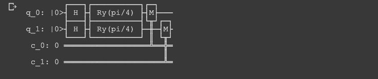

From this new distribution we can see that 01 and 10 are pretty much unchanged and 00 and 11 just flipped.

Now let's look at what happens if we wrap both the beginning and end of the circuit with Hadamard gates:

We can see that that the circuit output distribution is actually the same as our original state vector.

3.3 The Deutsch Jozsa algorithm in Qiskit

Now let's write our black box function to check if the output is balanced or constant.

To do this we:

• Use 2 CNOT gate for qubit 0 and qubit 1 to index 2
• Define a circuit with 3 qubits and 2 classical bits
• Apply Hadamard gates to both ends of the circuit
• Add a NOT gate to qubit 2 at the start of the circuit
• Measure qubit 0 and 1 and map them to classical bit 0 and 1

# black box function balanced & constant
def balanced_black_box(c):
  c.cx(0, 2)
  c.cx(1, 2)
  return c

def constant_black_box(c):
  return c

c = q.QuantumCircuit(3,2)
c.x(2)
c.barrier()
c.h(0)
c.h(1)
c.h(2)
c.barrier()
c = balanced_black_box(c)
c.barrier()
c.h(0)
c.h(1)
c.h(2)
c.measure([0,1], [0,1])
c.draw()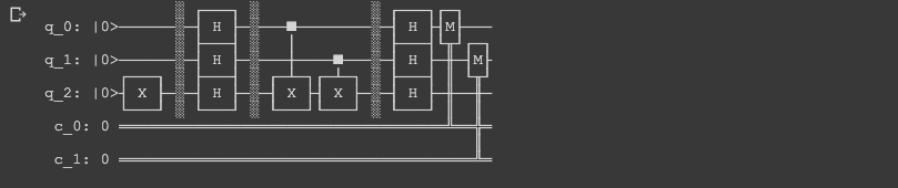

We can see we get 11 with the balanced black box and 00 with the constant black box:

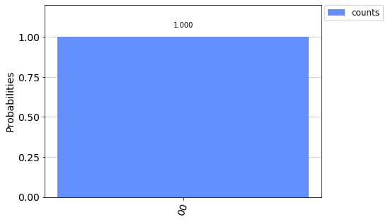
As mentioned, a classical computer would require two queries to answer this question, but with a quantum computer and superposition we only need one query to understand the variability of output.

Even though this is a relatively useless problem to solve, it does prove the speed advantage of quantum computing over classical computers.

Summary: Quantum Programming with Qiskit

In this guide we introduced quantum programming with Qiksit, the open-source framework for working with quantum computers.

We first discussed how to get started with Qiskit, how to define quantum circuits and gates, and finally how to program the Deutsch Jozsa Algorithm.

If you want to learn more about quantum programming and Qiskit check out the resources below.

Further Resources:

• Sentdex Tutorial
• Qiskit Education
• Qiskit Documentation
• Teach Me Quantum