Time Series with TensorFlow: Building a Convolutional Neural Network (CNN) for Forecasting

In this Time Series with TensorFlow article, we build a Conv1D (CNN) model for forecasting Bitcoin price data.

a year ago • 6 min read

By Peter Foy

So far in the Time Series with TensorFlow project we've created a total of 4 models, including a naive model and 3 dense models with varying window and horizon sizes.

As we've seen, our deep learning models have not outperformed our naive model (more on this below), so in this article we're going to continue testing models and build a convolutional neural network (CNN) for time series forecasting.

This article is based on notes from this TensorFlow Developer Certificate course and is organized as follows:

Autocorrelation & time series forecasting
Preparing our data for a Conv1D model
Model 4: Building a Conv1D model for forecasting

Previous articles in this series can be found below:

Stay up to date with AI

Autocorrelation & time series forecasting

As we compared the mean absolute error (MAE) of each model, however, we saw that the naive model was still outperforming our deep learning models.

One of the reasons the naive results are better could be due to the presence of autocorrelation in the data, which Investopedia defines as:

Autocorrelation represents the degree of similarity between a given time series and a lagged version of itself over successive time intervals.

Autocorrelation measures the relationship between a variable's current value and its past values.

In simpler terms, if take our daily Bitcoin price dataset, high autocorrelation just means the next day's price is going to be close to the previous day's price.

Since our naive model just predicts the next day's price will be the previous day, high autocorrelation is likely why it's outperforming our initial deep learning models.

A key takeaway from this is that although we can build deep learning models for time series forecasting, there are a number of pitfalls to avoid. If you want to learn more, check out this article on How (not) to use Machine Learning for time series forecasting: Avoiding the pitfalls.

That said, we've only built simple dense models so far, so in this article we're going to build a convolutional neural network (CNN) for time series forecasts.

Preparing our data for a Conv1D model

In order to prepare our data for a CNN model, we need to frame it as a seq2seq problem, or a "many to one" sequence problem as discussed earlier:

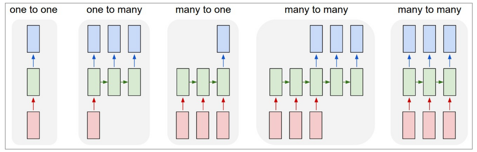
By formatting our data for a seq2seq problem, we can build both recurrent neural networks (RNNs) and 1-dimensional CNNs (Conv1D) models.

To start, let's set our global horizon and window sizes as follows:

HORIZON=1
WINDOW_SIZE=7

To recap, this just means we're using the previous 7-days of data to predict the next day's price.

Next, we'll create a windowed dataset with our make_windows() helper function as we've done before:

# Create windowed data
full_windows, full_labels = make_windows(prices, window_size=WINDOW_SIZE, horizon=HORIZON)
len(full_windows), len(full_labels)

Next we need to create train and test splits of our windowed data with our make_train_test_splits() function:

# Create train/test splits
train_windows, test_windows, train_labels, test_labels = make_train_test_splits(full_windows, full_labels)
len(train_windows), len(test_windows), len(train_labels), len(test_labels)

Let's now check out the TensorFlow docs for Conv1D models, which we see is a:

1D convolution layer (e.g. temporal convolution).

A "temporal convolution" just means that there is a time component, as is the case with our Bitcoin price data.

If we look at the input shape, we see we have a 3+D tensor with shape: batch_shape + (steps, input_dim)

Our data isn't in this shape yet, instead it's in this shape right now:

# Check data input shape
train_windows[0].shape # returns (WINDOW_SIZE, )

(7,)

Now what is the input_dim?

To recap, our model views 7 days of samples to predict the next day's price. This means we need to alter the input dimension to get it to (7, 1).

To do so, let's define a TensorFlow constant for our train_windows:

# Let's reshape our data to pass it into a Conv1D layer
x = tf.constant(train_windows[0])
x

Next, we'll create an expand_dims_layer as follows:

expand_dims_layer = layers.Lambda(lambda x: tf.expand_dims(x, axis=1)) # add an extra dimension for 'input_dims'

What this does is take our input Tensor with shape of (7,) and expands it by a dimension to make it (7, 1).

The Lambda layer in TensorFlow "wraps arbitrary expressions as a Layer object", which just means we can turn lambda expressions into a TensorFlow layer.

Let's now test our lamba layer:

# Test our lambda layer
print(f"Original shape: {x.shape}") # (WINDOW_SIZE)
print(f"Expanded shape: {expand_dims_layer(x).shape}")
print(f"Original values with expanded shape:\n {expand_dims_layer(x)}")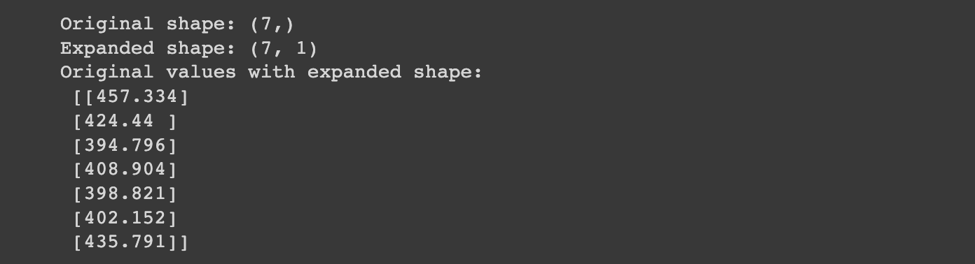

Now that have the expanded shape that we need for a Conv1D model, let's build the model.

Model 4: Building a Conv1D model for forecasting

In order to build our Conv1D model, we're going to need the following layers:

Lambda layer
Conv1D model with filters=128, kernel_size=7 (sliding window of 7), and padding="causal" (useful when modeling temporal data), activation="relu"
Output layer

# Model 4: Conv1D

tf.random.set_seed(42)

# Create Conv1D model
model_4 = tf.keras.Sequential([
    layers.Lambda(lambda x: tf.expand_dims(x, axis=1)),
    layers.Conv1D(filters=128, kernel_size=7, strides=1, padding="causal", activation="relu"),
    layers.Dense(HORIZON)
], name="model_4_conv1D")

# Compile model
model_4.compile(loss="mae",
                optimizer=tf.keras.optimizers.Adam())

# Fit model
model_4.fit(train_windows,
            train_labels,
            batch_size=128,
            epochs=100,
            verbose=0,
            validation_data=(test_windows, test_labels),
            callbacks=[create_model_checkpoint(model_name=model_4.name)])

Let's now get a summary, evaluate model_4, and load in the best performing model:

model_4.summary()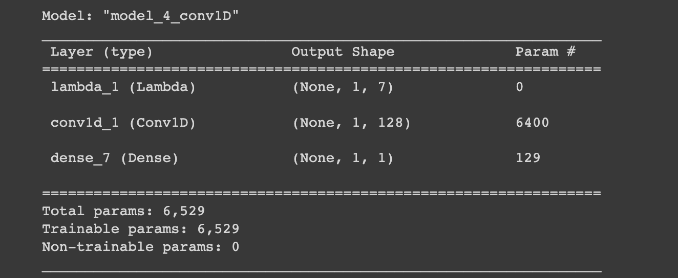

# Evaluate model
model_4.evaluate(test_windows, test_labels)

This gives us an MAE of 1180. If we load in the best performing model we get an MAE of 1121:

# Load in best performing model
model_4 = tf.keras.models.load_model("model_experiments/model_4_conv1D")
model_4.evaluate(test_windows, test_labels)

Let's now make predictions with our model:

# Make predictions
model_4_preds = make_preds(model_4, test_windows)
model_4_preds[:10]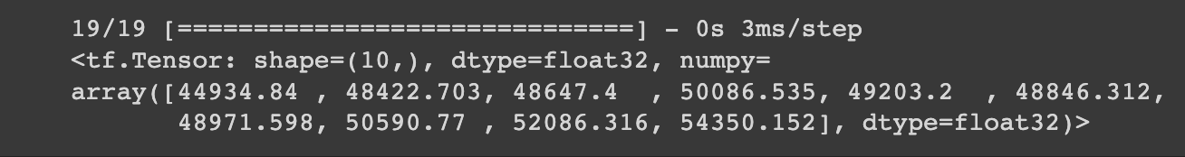

Let's now evaluate these predictions:

# Evaluate predictions
model_4_results = evaluate_preds(y_true=tf.squeeze(test_labels),
                                 y_pred=model_4_preds)
model_4_results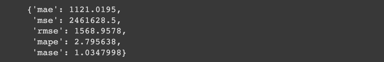

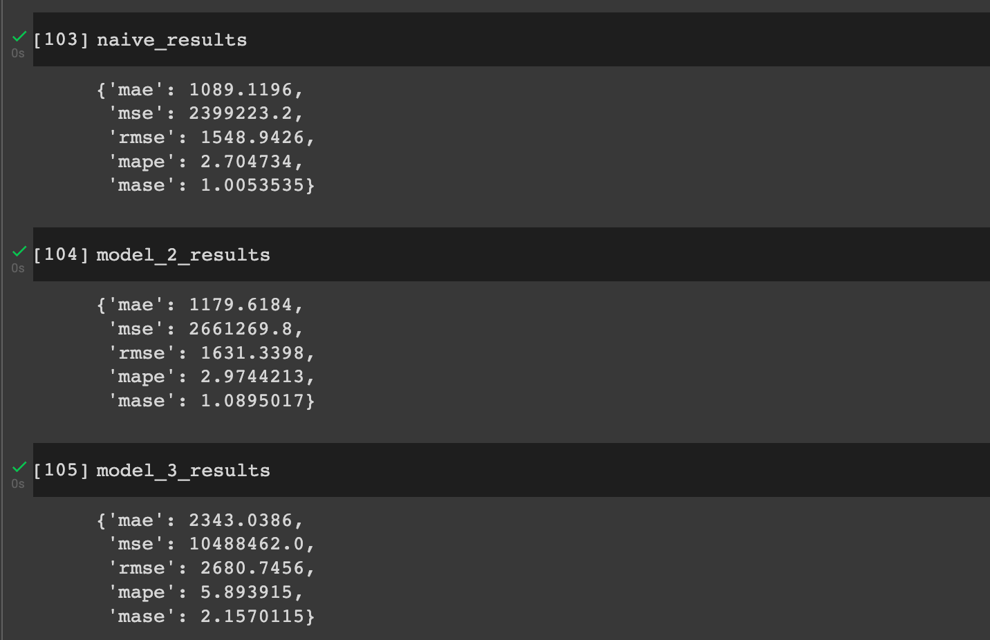
Let's check how these compare to our naive results and previous models:

Summary: Building a Conv1D model for forecasting

In this article, we first discussed autocorrelation in time series forecasting. We then discussed how to prepare our data for a Conv1D model by expanding the shape of our input dimensions. Finally, we built a simple Conv1D model and evaluated the results.

We can see the Conv1D model is performing better than our previous dense models, but still not as good as our naive model. Of course, we could try and improve the Conv1D results by training for longer, tuning our model hyperparameters, and so on.

For now, we'll skip hyperparameter tuning and continue building new models. In the next article, we create an LSTM (RNN) model for time series forecasting.