

In the previous article, we turned our data into a windowed time series in order to turn the forecasting problem into a supervised learning problem.
In this article, we're going to create our first deep learning model for time series forecasting, but first, we need to create a modeling checkpoint callback to save our best performing models.
This article is based on notes from this TensorFlow Developer Certificate course and is organized as follows:
- Create a modeling checkpoint callback
- Model 1: Building our first deep learning model for Bitcoin price forecasting
- Creating a function to make predictions with our trained models
- Make predictions with
model_1on test data
Previous articles in this series can be found below:
- Time Series with TensorFlow: Downloading & Formatting Historical Bitcoin Data
- Time Series with TensorFlow: Building a Naive Forecasting Model
- Time Series with TensorFlow: Common Evaluation Metrics
- Time Series with TensorFlow: Formatting Data with Windows & Horizons
Stay up to date with AI
Create a modeling checkpoint callback
Since our model's performance will fluctuate from experiment to experiment, we want to create a model checkpoint to compare models more efficiently.
More specifically, epoch to epoch the performance of each model will change, so we want to compare each of our model's best performance against the other model's best performance.
For example, if the model performs the best on epoch 50 but we train it for 100 epochs, we want to load and evaluate the model saved on epoch 50.
That is what a modelling checkpoint callback does.
We can find TensorFlows docs for model checkpoints here: tf.keras.callbacks.ModelCheckpoint.
With this callback we have save_best_only which accomplishes the task of saving the model when it's considered the best.
Here's the code we'll use to create a modeling checkpoint:
import os

# Create a function to implement a ModelCheckpoint callback
def create_model_checkpoint(model_name, save_path="model_experiments"):
  return tf.keras.callbacks.ModelCheckpoint(filepath=os.path.join(save_path, model_name),
                                            verbose=0,
                                            save_best_only=True)
Model 1: Building our first deep learning model for Bitcoin price forecasting
We've now pre-processed and prepared our data for forecasting, it's time to start building our first model.
The first model we'll build is a dense model with a window size of 7 and a horizon of 1. As discussed, this simply means we're using a week's worth of data in order to predict the next day's price.
Below are the model parameters of our first dense model:
- A single dense layer with 128 hidden units and ReLU activation
- An output layer with linear activation (note this is the same as having no activation)
- An Adam optimizer and MAE loss function
- A batch size of 128
- Run for 100 epochs
Of course, it's highly unlikely these hyperparameters will be optimal, but it'll give us another base to improve upon in future models.
import tensorflow as tf
from tensorflow.keras import layers
tf.random.set_seed(42)
# 1. Construct model
model_1 = tf.keras.Sequential([
layers.Dense(128, activation="relu"),
layers.Dense(HORIZON, activation="linear")
], name="model_1_dense")
# 2. Compile model
model_1.compile(loss="mae",
optimizer=tf.keras.optimizers.Adam(),
metrics=["mae"])
# 3. Fit model
model_1.fit(x=train_windows,
y=train_labels,
epochs=100,
verbose=1,
batch_size=128,
validation_data=(test_windows, test_labels),
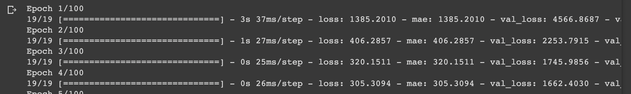
callbacks=[create_model_checkpoint(model_name=model_1.name)])For this model, we can see the MAE starts ~1386 and ends at ~178.
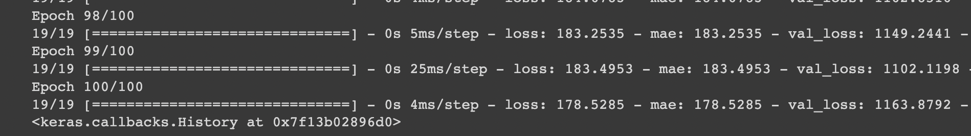
Let's now evaluate model 1 on test data, which returns an MAE of 1163.
# Evaluate model on test data
model_1.evaluate(test_windows, test_labels)
Now let's use our model checkpoint callback and load in the best performing model and evaluate it on test data:
# Load in saved best perfomring model_1 and evaluate it on test data
model_1 = tf.keras.models.load_model("model_experiments/model_1_dense")
model_1.evaluate(test_windows, test_labels)
In this case, our best performing model returns an MAE of 1102. If you recall, the MAE of our naive results was 1089, so this isn't yet doing better than the naive model.
Before building another model, let's first create a function to make predictions with our trained model.
Creating a function to make predictions with our trained models
If you recall, with our time-series data split we're only making pseudo forecasts as the test data isn't actually in the future. This means our test results are also only a partial representation of how the model may perform in real time series forecasting.
That said, let's write a function to create pseudo-forecasts on the test data with our trained models. The model will:
- Take in a trained model
- Take in some input data (the same kind of data the model was trained on)
- Passes the input data to the model's
predict()method - Returns the predictions
def make_preds(model, input_data):
  """
  Uses model to make predictions on input_data.
  """
  forecast = model.predict(input_data)
  return tf.squeeze(forecast) # return 1D array of predictions
Make predictions with model_1 on test data
Let's now use our function and make predictions using our best-performing model_1:
model_1_preds = make_preds(model_1, test_windows)
len(model_1_preds), model_1_preds[:10]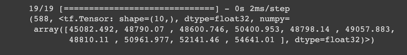
We can now evaluate these forecasts with our evaluate_preds() function:
model_1_results = evaluate_preds(y_true=test_labels, y_pred=model_1_preds)
model_1_results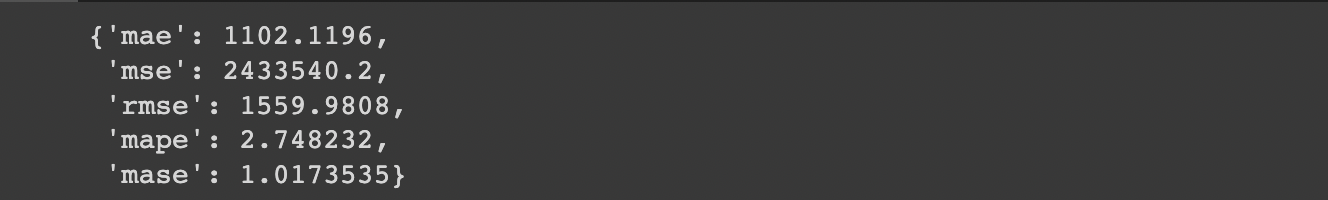
Let's compare these to our naive results:
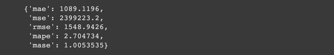
As we can see our naive model slightly beat our first deep learning model on every metric.
Before building a new model, let's first plot our model_1 predictions:
# Plot model_1 predictions
offset = 300
plt.figure(figsize=(10, 7))

# Account for the test_window offset and index into test_labels to ensure correct plotting
plot_time_series(timesteps=X_test[-len(test_windows):],
                 values=test_labels[:, 0], start=offset, label="Test_data")

plot_time_series(timesteps=X_test[-len(test_windows):],
                 values=model_1_preds, start=offset, format="-", label="model_1_preds")
Summary: Building our first deep learning forecasting model
In this article, we started by creating a modeling checkpoint callback so that we can s compare each of our best performing models against each other.
We then build a simple dense model for time series forecasting, which we saw did slightly worse than our naive results.
Now that we've completed our first modeling experiment, in the next article, we'll expand on this with the same architecture but test different window sizes and horizons.


