Time Series with TensorFlow: Building dense models with larger windows & horizons

In this article, we build two dense models with larger window & horizon sizes.

a year ago • 7 min read

By Peter Foy

In our previous time series with TensorFlow article, we created our first deep learning model for Bitcoin price forecasting.

As we saw, this first model didn't perform as well as the naive model, so in this article we'll expand on it by adjusting the window and horizon size while keeping the same model architecture.

In particular, we'll test two models with a window size of 30 and a horizon of 1, and a window size of 30 with a horizon of 7. This article is based on notes from this TensorFlow Developer Certificate course and is organized as follows:

Model 2: Dense (window = 30, horizon = 1)
Evaluating Model 2
Model 3: Building a model with a larger horizon
Adjusting our evaluation function to work with larger horizons
Visualizing model 3 results

Previous articles in this series can be found below:

Stay up to date with AI

Model 2: Dense (window = 30, horizon = 1)

We previously set our window and horizon global variables to 7 and 1, so let's first adjust these variables:

HORIZON=1
WINDOW_SIZE=30

Next, we'll make windowed data with the appropriate horizon and window sizes.

To do so, we need to recreate our full_windows and full_labels variables with our make_windows function, which "turns a 1D array into a 2D array of sequential windows of window_size":

full_windows, full_labels = make_windows(prices, window_size=WINDOW_SIZE, horizon=HORIZON)

Next, we need to make train and test windows with our make_train_test_split() function:

# Make train & testing windows
train_windows, test_windows, train_labels, test_labels = make_train_test_splits(windows=full_windows, labels=full_windows, test_split=0.2)

Now that our data is prepared with the new window and horizon size, let's build a model with the same architecture as model_1:

tf.random.set_seed(42)

# Create model
model_2 = tf.keras.Sequential([
    layers.Dense(128, activation="relu"),
    layers.Dense(HORIZON)  
], name="model_2_dense")

# Compile model
model_2.compile(loss="mae",
                optimizer=tf.keras.optimizers.Adam())

# Fit model
model_2.fit(train_windows,
            train_labels,
            epochs=100,
            batch_size=128,
            validation_data=(test_windows, test_labels),
            callbacks=[create_model_checkpoint(model_name=model_2.name)])

Let's now evaluate model 2 on test data and then load in the best performing model:

# Evaluate model 2 on test data
model_2.evaluate(test_windows, test_labels)

# Load in best performing model
model_2 = tf.keras.models.load_model("model_experiments/model_2_dense")
model_2.evaluate(test_windows, test_labels)

Evaluating Model 2

Let's now get model 2's forecast predictions with our make_preds helper function:

# Get forecast predictions
model_2_preds = make_preds(model_2, input_data=test_windows)

We'll then evaluate the results of model_2's predictions:

# Evaluate results for model 2 predictions
model_2_results = evaluate_preds(y_true=tf.squeeze(test_labels), # remove 1 dimension of test labels
                                 y_pred=model_2_preds)
model_2_results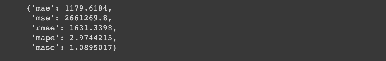

If you recall, our model_1 MAE was 1102 so it looks like adding a larger window size has performed worse. Let's still plot model 2's results with our plot_time_series function:

offset = 300
plt.figure(figsize=(10, 7))

# Account for test_window offset when plotting
plot_time_series(timesteps=X_test[-len(test_windows):], values=test_labels[:, 0], start=offset, label="test data")
plot_time_series(timesteps=X_test[-len(test_windows):], values=model_2_preds, start=offset, format="-", label="model 2 preds")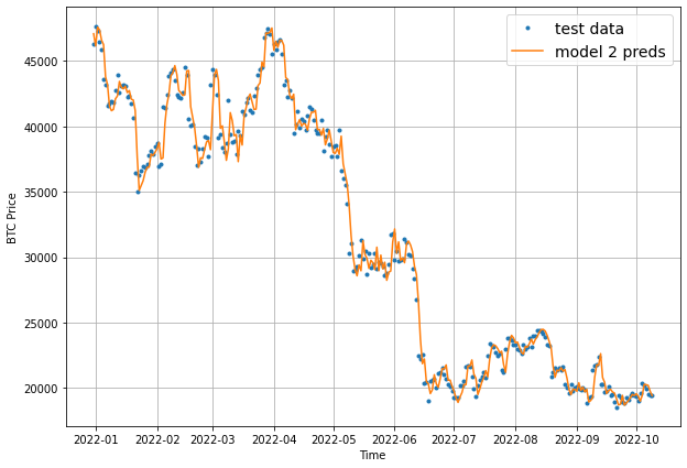

Model 3: Building a model with a larger horizon

In this model let's build another dense model with a window of 30, but with a larger horizon of 7.

To start, we need to change our global window and horizon variables, and then create our full_windows and full_labels with our make_windows() helper function:

HORIZON = 7
WINDOW_SIZE = 30

full_windows, full_labels = make_windows(prices, window_size=WINDOW_SIZE, horizon=HORIZON)
len(full_windows), len(full_labels)

Next, we'll create our train and test splits:

train_windows, test_windows, train_labels, test_labels = make_train_test_splits(windows=full_windows, labels=full_labels, test_split=0.2)
len(train_windows), len(test_windows), len(train_labels), len(test_labels)

Now we'll build the same model architecture as above, just with one slight difference. Since the horizon is larger we need to change the output shape of the model:

tf.random.set_seed(42)

# Create model
model_3 = tf.keras.Sequential([
    layers.Dense(128, activation="relu"),
    layers.Dense(HORIZON)
], name="model_3_dense")

# Compile model
model_3.compile(loss="mae",
                optimizer=tf.keras.optimizers.Adam())

# Fit model
model_3.fit(train_windows,
            train_labels,
            batch_size=128,
            epochs=100,
            verbose=0,
            validation_data=(test_windows, test_labels),
            callbacks=[create_model_checkpoint(model_name=model_3.name)])

Let's now evaluate model 3:

# Evaluate model on the test data
model_3.evaluate(test_windows, test_labels)

Here we can see the loss is much higher than previous models.

If we think about this logically, it makes sense that this model performs worse as it's predicting further into the future, which is of course a more difficult challenge (think predicting the next hour of weather vs. the next week).

That said, let's still evaluate model 3's best performing model with our helper function:

# Load best version of model_3 and evaluate
model_3 = tf.keras.models.load_model("model_experiments/model_3_dense")
model_3.evaluate(test_windows, test_labels)

Let's now make predictions with our model:

# Make predictions with model_3
model_3_preds = make_preds(model_3,
                           input_data=test_windows)
model_3_preds[:5]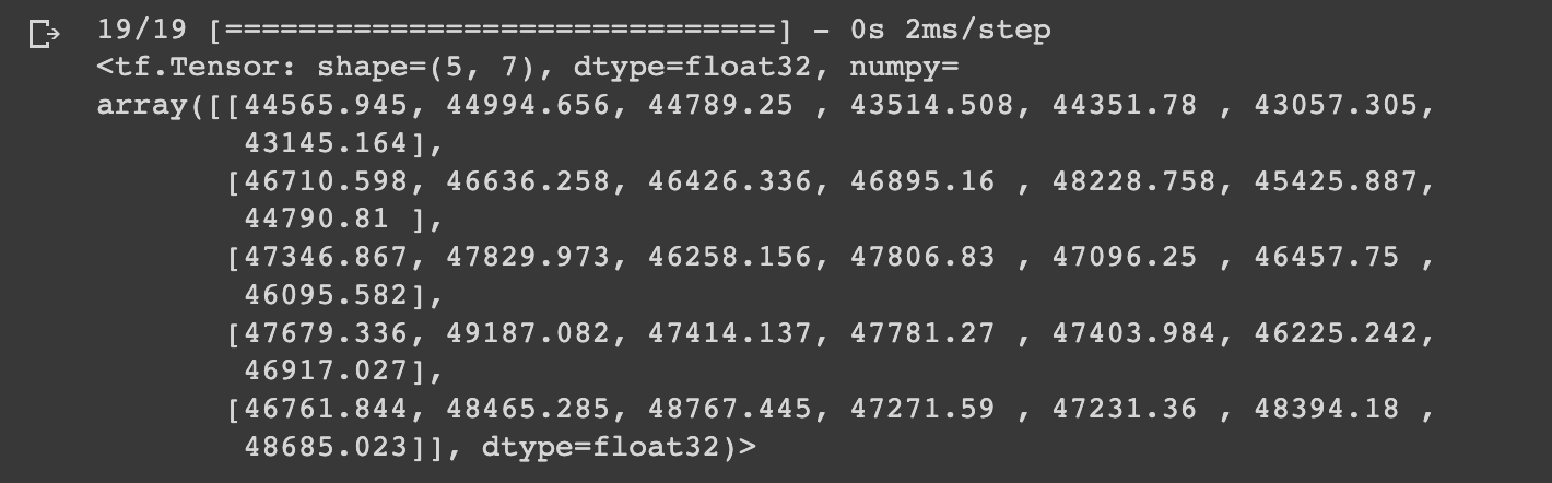

As expected, you'll notice with model_3 we have a shape of (5, 7), whereas with model_2 we had a shape of (5, 1).

Let's now evaluate model_3 results. If we just use the evaluate_preds function as before, we can see it outputs an array of multiple values for every metric.

# Evaluate model_3 results
model_3_results = evaluate_preds(y_true=tf.squeeze(test_labels),
                                 y_pred=model_3_preds)
model_3_results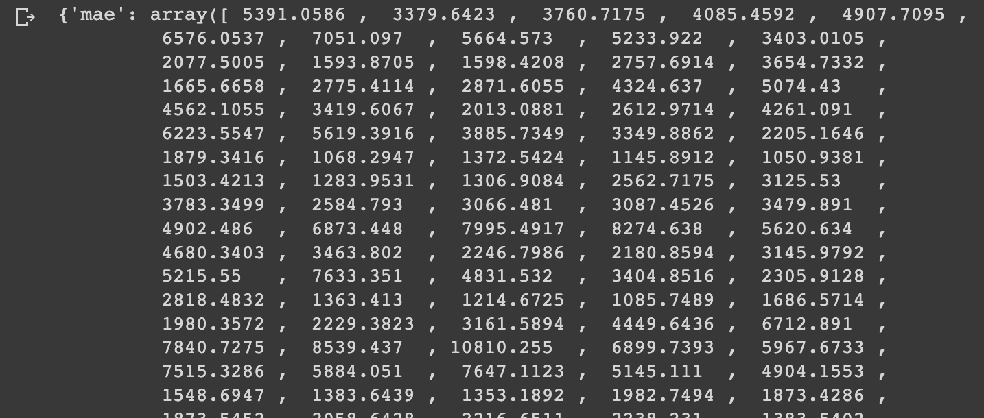

The reason for this is of course the different dimensionality with our new horizon size:

model_3_preds.shape, model_2_preds.shape

To solve this, we need to adjust our evaluate_preds function to work with our larger horizon size.

Adjusting our evaluation function to work with larger horizons

As mentioned, with model_3 we're getting a value for every value in the test dataset, as opposed to a single evaluation metric.

We need a way to aggregate this array of multiple values into a single value. To so do, we'll adjust our evaluate_preds() helper function to work with multiple dimensions.

You can find the original evaluate_preds() function below:

# Create a function to evaluate model forecasts with various metrics
def evaluate_preds(y_true, y_pred):
  # make sure float32 datatype
  y_true = tf.cast(y_true, dtype=tf.float32)
  y_pred = tf.cast(y_pred, dtype=tf.float32)

  # calculate various evaluation metrics
  mae = tf.keras.metrics.mean_absolute_error(y_true, y_pred)
  mse = tf.keras.metrics.mean_squared_error(y_true, y_pred)
  rmse = tf.sqrt(mse)
  mape = tf.keras.metrics.mean_absolute_percentage_error(y_true, y_pred)
  mase = mean_absolute_scaled_error(y_true, y_pred)

  return {"mae": mae.numpy(),
          "mse": mse.numpy(),
          "rmse": rmse.numpy(),
          "mape": mape.numpy(),
          "mase": mase.numpy()}

In order to update this to work with multiple dimensions, let's first look at the output of our evaluation metrics, such as MAE:

model_3_results["mae"].shape

(582,)

Comparing this to model_2_results["mae"].shape, we see it doesn't have a shape because it's a scalar value. If we compare the number of dimensions of each we see that model_3 has 1 dimension and model_2 has 0.

In order to account for different sized metrics (i.e. for longer horizon sizes), we're going to reduce metrics to a single dimension with an if statement and tf.reduce_mean and then return them as numpy arrays:

# Create a function to evaluate model forecasts with various metrics
def evaluate_preds(y_true, y_pred):
  # make sure float32 datatype
  y_true = tf.cast(y_true, dtype=tf.float32)
  y_pred = tf.cast(y_pred, dtype=tf.float32)

  # calculate various evaluation metrics
  mae = tf.keras.metrics.mean_absolute_error(y_true, y_pred)
  mse = tf.keras.metrics.mean_squared_error(y_true, y_pred)
  rmse = tf.sqrt(mse)
  mape = tf.keras.metrics.mean_absolute_percentage_error(y_true, y_pred)
  mase = mean_absolute_scaled_error(y_true, y_pred)

  # Account for different sized metrics
  if mae.ndim > 0:
    mae = tf.reduce_mean(mae)
    mse = tf.reduce_mean(mse)
    rmse = tf.reduce_mean(rmse)
    mape = tf.reduce_mean(mape)
    mase = tf.reduce_mean(mase)

  return {"mae": mae.numpy(),
          "mse": mse.numpy(),
          "rmse": rmse.numpy(),
          "mape": mape.numpy(),
          "mase": mase.numpy()}

If we now run evaluate_preds on model 3 we get the following results:

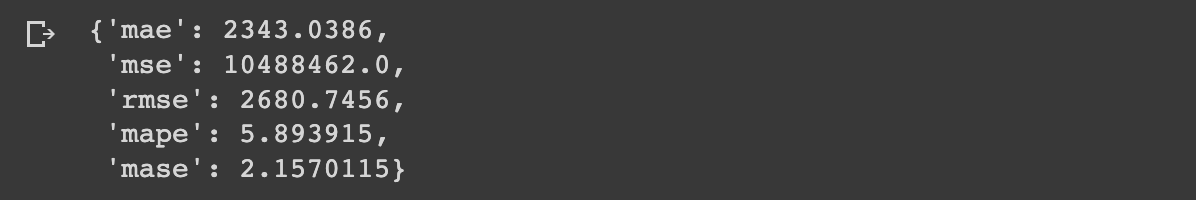
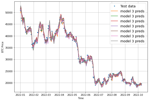
Visualizing model 3 results

To finish off this model, let's now visualize the results. Once again, we need to aggregate the results of model_3 preds, otherwise we get this:

To resolve this, we'll use tf.reduce_mean() and set the axis to 1 as follows:

offset = 300
plt.figure(figsize=(10, 7))
# Account for test_window offset when plotting
plot_time_series(timesteps=X_test[-len(test_windows):], values=test_labels[:, 0], start=offset, label="Test data")
plot_time_series(timesteps=X_test[-len(test_windows):], values=tf.reduce_mean(model_3_preds, axis=1), start=offset, format="-", label="model 3 preds")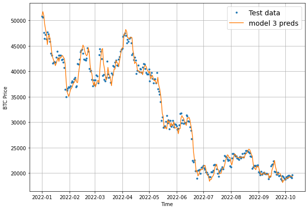

Keep in mind that we've now aggregated the 7-day forecast into a singular value so we will lose some information in our visualization.

Summary: Increasing our window & horizon size

In this article, we looked at how to build two dense models with larger window and horizon sizes.

We saw that as we increased the horizon size the model performed significantly worse, although that makes sense since making predictions further into the future is much more challenging and we kept the model architecture the same.

In the following articles, we'll move beyond our simple dense model and build a convolutional neural network (CNN) and recurrent neural network (RNN) for time series forecasting.