

In our previous articles in this series on Time Series with TensorFlow, we've built simple dense models, CNNs, RNNs, and replicated the N-BEATS algorithm.
Even with all this added complexity, we still haven't been able to beat the results of our naive model when it comes to the task of forecasting the price of Bitcoin.
Despite that, in this article, we're going to put several models together and build an ensemble model.
An ensemble model can be thought of as simply multiple models stacked together.
Ensemble models can increase the overall predictive performance by combining the strengths of individual models and reducing their weaknesses.
This article is based on notes from this TensorFlow Developer course and is organized as follows:
- Constructing and fitting an ensemble of models using different loss functions
- Making and evaluating predictions with our ensemble model
Stay up to date with AI
Constructing and fitting an ensemble of models using different loss functions
In this Time Series with Tensorflow series we've been attempting to predict the price of Bitcoin, so we're going to build multiple models all with that goal.
To recap, our HORIZON (i.e. forecasting window) is 1 day and our WINDOW_SIZE is 7.
First, we're going to write a function called get_ensemble_models that will return a list of trained models that use different loss functions, which will
- Make an empty list of trained ensemble models
- Create
num_iternumber of models per loss function - Build and fit a new model with a new loss function
- Construct a simple model (similar to model_1) - one new parameter we will add is
kernel_initializer="he_normal", which as the docs say, initializes the model with a normal gaussian distribution. - Compile the simple model with the current loss function
- Fit the current model
- Append fitted model to list of ensemble models
def get_ensemble_models(horizon=HORIZON,
train_data=train_dataset,
test_data=test_dataset,
num_iter=10,
num_epochs=1000,
loss_fn=["mae", "mse", "mape"]):
"""
Returns a list of num_iter models each trained on MAE, MSE, and MAPE loss.
For example, if num_iter=10, a list of 30 trained models will be returned:
10 * len(["mae", "mse", "mape"]).
"""
# Make empty list for trained ensemble models
ensemble_models = []
# Create num_iter number of models per loss function
for i in range(num_iter):
# Build and fit a new model with a new loss function
for loss_function in loss_fns:
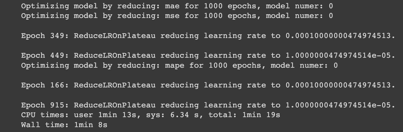
print(f"Optimizing model by reducing: {loss_function} for {num_epochs} epochs, model numer: {i}")
# Construct a simple model (similar to model_1)
model = tf.keras.Sequential([
# Initalize dense layers with normal distribution for estimating prediction intervals
layers.Dense(128, kernel_initializer="he_normal", activation="relu"),
layers.Dense(128, kernel_initializer="he_normal", activation="relu"),
layers.Dense(HORIZON)
])
# Compile simple model with current loss function
model.compile(loss=loss_function,
optimizer=tf.keras.optimizers.Adam(),
metrics=["mae", "mse"])
# Fit the current model
model.fit(train_data,
epochs=num_epochs,
verbose=0,
validation_data=test_data,
callbacks=[tf.keras.callbacks.EarlyStopping(monitor="val_loss",
patience=200,
restore_best_weights=True),
tf.keras.callbacks.ReduceLROnPlateau(monitor="val_loss",
patience=100,
verbose=1)])
# Append fitted model to list of ensemble models
ensemble_models.append(model)
return ensemble_modelsNext, let's run this function as follows:
%%time
# Get list of trained ensemble models
ensemble_models = get_ensemble_models(num_iter=5,
                                      num_epochs=1000)
Making and evaluating predictions with our ensemble model
Next, let's make and evaluate predictions with our ensemble model.
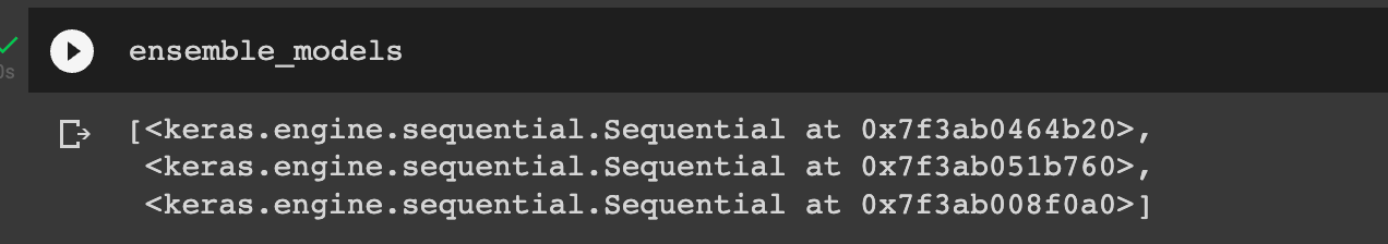
Now let's look at each of our ensemble_models we see we have 3 trained models:
Let's make some predictions with these models - to do so we'll create a function that uses a list of trained models to make and return a list of predictions:
def make_ensemble_preds(ensemble_models, data):
  ensemble_preds = []
  for model in ensemble_models:
    preds = model.predict(data)
    ensemble_preds.append(preds)
  return tf.constant(tf.squeeze(ensemble_preds))
Next, we'll create a list of ensemble predictions:
# Create a list of ensemble predictions
%%time
ensemble_preds = make_ensemble_preds(ensemble_models=ensemble_models,
                                     data=test_dataset)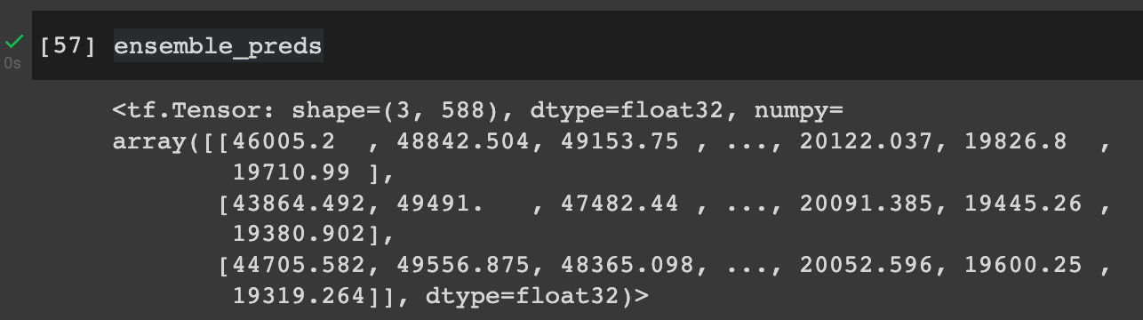
Now, let's evaluate these predictions with our evaluate_preds helper function from a previous article:
evaluate_results = evaluate_preds(y_true=y_test,
                                  y_pred=ensemble_preds)
evaluate_results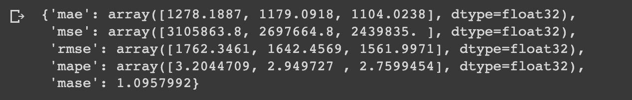
From MachineLearningMastery's article on combining predictions for ensemble learning:
Combining numerical predictions often involves using simple statistical methods; for example: Mean Predicted Value and Median Predicted Value. Both give the central tendency of the distribution of predictions.
Let's take the mean of our ensemble results:
ensemble_mean = tf.reduce_mean(ensemble_preds, axis=0)
ensemble_mean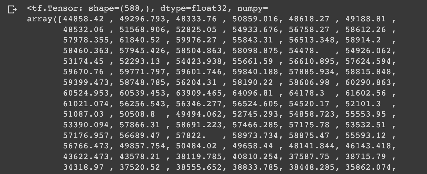
Now let's get the median:
ensemble_median = np.median(ensemble_preds, axis=0)
ensemble_median[:10]
Now if we reduce the mean or median before passing it into our evaluate_preds function we see a significant reduction in MAE:
evaluate_results = evaluate_preds(y_true=y_test,
                                  y_pred=ensemble_mean)
evaluate_results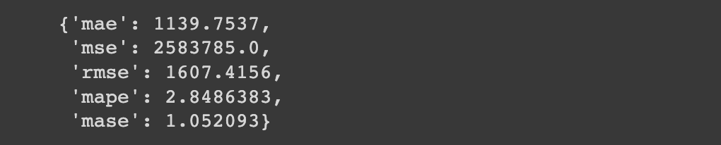
It is still higher than our naive results and is roughly the same as the performance of the N-BEATS algorithm in our previous article.
Summary: Ensemble Learning for Time Series Forecasting
In this article, we saw how we can use ensemble learning to train multiple machine learning models for the task of time series forecasting and combine their predictions to improve performance.
To do this, we constructed and fit an ensemble of models using different loss functions. We then made predictions and evaluated our results, which we saw performed similarly to the N-BEATS algorithms.
In the next article, we'll discuss how we can take our ensemble model and get a range of prediction intervals.


