

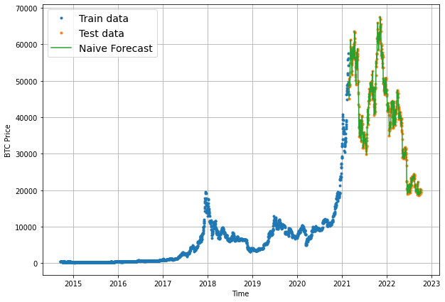
In the previous article in this series, we built our first naive forecasting model for Bitcoin prices and can see visually it follows the test data quite closely. In this article, we'll quantify how accurate it is with several common time series evaluation metrics.
This article is based on notes from this TensorFlow Developer Certificate course and is organized as follows:
- Common Time Series Evaluation Metrics
- Implementing MASE with TensorFlow
- Creating a function to evaluate our model's forecasts
Common Time Series Evaluation Metrics
Since we're predicting a number with our forecasting models, this means we working on a regression problem. Given this, we'll need some regression metrics to evaluate the models.
A few of the most common time series evaluation metrics include:
- MAE: Mean absolute error - this s a great starter metric for any regression problem.
tf.keras.losses.MAE() - MSE: Mean squared error - this is useful when larger errors are more significant than smaller errors.
tf.keras.losses.MSE() - Huber Loss: Combination of MAE and MSE - less sensitive to outliers than MSE.
- MASE: Mean absolute scaled error - a scaled error is >1 if the forecast is worse than the naive ad <1 if the forecast is better than the naive. Requires custom code or sktime's
mase_loss().
To recap, with these metrics the main thing we're evaluating is how our model's forecast (y_pred) compare to the actual values (y_true).
Also, given that we're working with non-seasonal time series data, we're going to work with the non-seasonal version of MASE, which as Forecasting: Principles and Practice highlights:
...a useful way to define a scaled error uses naïve forecasts.
Mathematically, we can write the equation we'll be coding next as:
$$q_j = \frac{e_j}{\frac{1}{T-1}\sum\limits^T_{t=2}|y_t - y_{t-1}|}$$
Stay up to date with AI
Implementing MASE with TensorFlow
Let's now see how we can implement MASE with TensorFlow. After that, we'll write a function to evaluate our models with various metrics.
As mentioned, sktime (scikit-learn for time series) has an implementation of MASE that we can take inspiration from. If we check GitHub we can also find a NumPy implementation here.
Below is the implementation we'll be using for this project:
# MASE implementation
def mean_absolute_scaled_error(y_true, y_pred):
  """
  Implement MASE (assuming no seasonality of data)
  """
  mae = tf.reduce_mean(tf.abs(y_true-y_pred))

  # Find MAE of naive forecast (no seasonality)
  mae_naive_no_season = tf.reduce_mean(tf.abs(y_true[1:] - y_true[:-1])) # our seasonality is 1 day, hence the shift of 1

  return mae / mae_naive_no_season
Let's see this in practice, which we can see is very close to 1 (the difference is due to the precision in computing):
mean_absolute_scaled_error(y_true=y_test[1:], y_pred=naive_forecast).numpy()Going forward, if our MASE is lower than this the model is better than the naive forecast and if it's higher it's worse than naive.
Creating a function to evaluate forecasts with various metrics
Let's now create a function to evaluate our time series forecasts with the following metrics:
- MAE
- MSE
- RMSE
- MAPE
- MASE
The function takes in model predictions and true values and returns a dictionary of evaluation metrics.
Next, we want to ensure our datatypes are float32 for metric calculations as TensorFlow will sometimes return errors without this.
After that we will calculate all the evaluation metrics mentioned above as follows:
# Create a function to evaluate model forecasts with various metrics
def evaluate_preds(y_true, y_pred):
  # Make sure float32 datatype
  y_true = tf.cast(y_true, dtype=tf.float32)
  y_pred = tf.cast(y_pred, dtype=tf.float32)

  # Calculate various evaluation metrics
  mae = tf.keras.metrics.mean_absolute_error(y_true, y_pred)
  mse = tf.keras.metrics.mean_squared_errory(y_true, y_pred)
  rmse = tf.sqrt(mse)
  mape = tf.keras.metrics.mean_absolute_percentage_error(y_true, y_pred)
  mase = mean_absolute_scaled_error(y_true, y_pred)

  return {"mae": mae.numpy(),
          "mse": mse.numpy(),
          "rmse": rmse.numpy(),
          "mape": mape.numpy(),
          "mase": mase.numpy()}
Let's now see if the function works with our naive results:
naive_results = evaluate_preds(y_true=y_test[1:],
                               y_pred=naive_forecast)
naive_results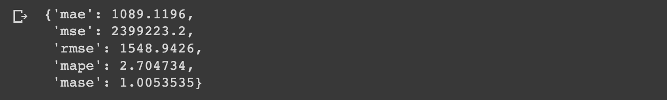
If we just look at the mae result, this is saying that the naive forecast on average was $1089 off from the true price of Bitcoin. Also, keep in mind that predictions on y_test only give us a hint of how our model might perform in the future since this data is still in the past.
Summary: Time Series Evaluation Metrics
In this article, we discussed several common time series evaluation metrics to evaluate our naive forecasting model.
In addition to the evaluation metrics that come built into TensorFlow, we also saw how we can implement another evaluation metric: mean absolute squared error (MASE).
Finally, we wrote a function to easily calculate these metrics and compare the performance of future models against the naive forecast.
In the next article, we'll continue formatting our data and discuss how to use windows and horizons in time series data.


