

In the previous article in this Time Series with TensorFlow series, we downloaded historical Bitcoin price data and then split it into training and test sets for modeling.
In this article, we'll discuss the various modeling experiments we'll be running, as well as build a naive forecasting model for daily Bitcoin price data.
This article is based on notes from this TensorFlow Developer Certificate course and is organized as follows:
- Modeling experiments
- Making a naive forecasting model
Stay up to date with AI
Modeling experiments
Now that we have our data ready, we'll run a series of modeling experiments to see which one performs best.
Naive Model
The purpose of building a naive model is to simply have a baseline to measure our more complex models against.
Dense Model
We will create several dense models with different window sizes.
Conv1D
Conv1D models can be used for sequence models so we will test this.
LSTM
LSTMs are another sequence model that falls under the family of recurrent neural networks (RNNs).
N-BEATS Algorithm
The N-BEATs algorithm is a univariate times series forecasting model that uses deep learning.
Ensemble Model
Ensemble models stack multiple models together to create a prediction.
Making a naive forecasting model
As mentioned, the reason to build a naive forecasting model first is to have a baseline to measure future models against. As highlighted in the book Forecasting: Principles and Practice:
Some forecasting methods are extremely simple and surprisingly effective.
There are several simple forecasting methods highlighted in this section of the book. The method we'll use is the naïve forecast where we simply set all forecasts to the value of the last observation.
Mathematically we can write this as:
$$\hat{y}_{T+h|T} = y_T$$
In simple terms, this means the prediction at timestep $t$ or $\hat{y}_{T+h|T}$ is equal to the value at the previous timestep $ y_T$.
We can write this out in code easily as follows:
# Create naive forecast
naive_forecast = y_test[:-1]
If we look at these values, we see that with a horizon of 1 the naive forecast is simply predicting the previous timestep as the next steps value.
Let's plot the naive forecast predictions with the plotting method we created in the previous article. Note we need to offset X_test by 1 for our naive forecast plot since it won't have a value for the first timestep.
plt.figure(figsize=(10,7))
plot_time_series(timesteps=X_train, values=y_train, label="Train data")
plot_time_series(timesteps=X_test, values=y_test, label="Test data")
plot_time_series(timesteps=X_test[1:], values=naive_forecast, format="-", label="Naive Forecast")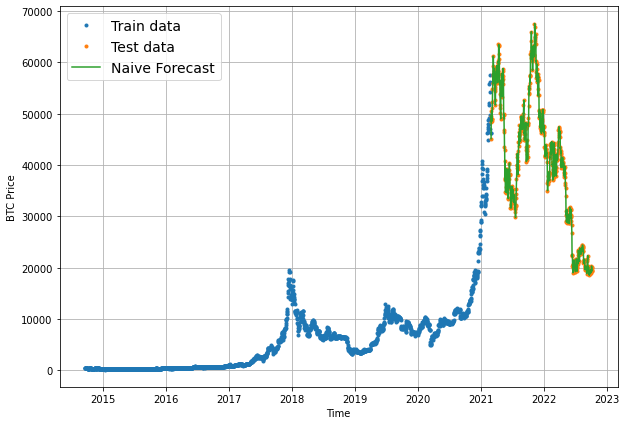
We can see the naive forecast follows the test data quite closely. This makes sense since we're not actually building a model, we're just offsetting the y_test values by 1 index. As we'll see building future models, it's actually quite difficult to beat this naive forecast baseline.
Before we start building more complex models, in the next article we'll discuss several common time series evaluation metrics.
Summary: Naive Forecasting with Time Series Data
In this article, we discussed the time series modeling experiments we'll be building and then built a simple naive forecast as a baseline.
The naive forecast we built simply predicted the next value to be the value at the previous timestep. In other words, the prediction at timestep $t$ is equal to the value at the previous timestep $ y_T$.


