

In previous articles in this Time Series with TensorFlow series, we've now built 8 models, ranging from simple dense models, CNNs, RNNs, we've replicated the N-BEATs algorithm, and put multiple models together with ensemble learning.
With each of these models, however, we've been forecasting a single value for the future price of Bitcoin, in other words, we've been making point predictions.
In this article, we'll discuss a key concept in forecasting: prediction intervals, which are also referred to as uncertainty estimates.
Instead of single point values, prediction intervals give us a range of prediction values with upper and lower bounds.
This article is based on notes from this TensorFlow Developer course and is organized as follows:
- The importance of prediction intervals in forecasting
- Getting the upper & lower bounds of our prediction interval
- Plotting prediction intervals of our ensemble model
Stay up to date with AI
The importance of prediction intervals in forecasting
Given the uncertainty associated with time series forecasting, using prediction intervals instead of single point estimates is very common in practice.
For example, in this article on Engineering Uncertainty Estimation in Neural Networks for Time Series Prediction at Uber, they state that:
Uncertainty estimation in deep learning remains a less trodden but increasingly important component of assessing forecast prediction truth in LSTM models.
In the image below, we see they've created a forecasting model where the...
"True values are represented by the orange line, and predictions by the blue dashed line, where the 95 percent prediction band is shown as the grey area":
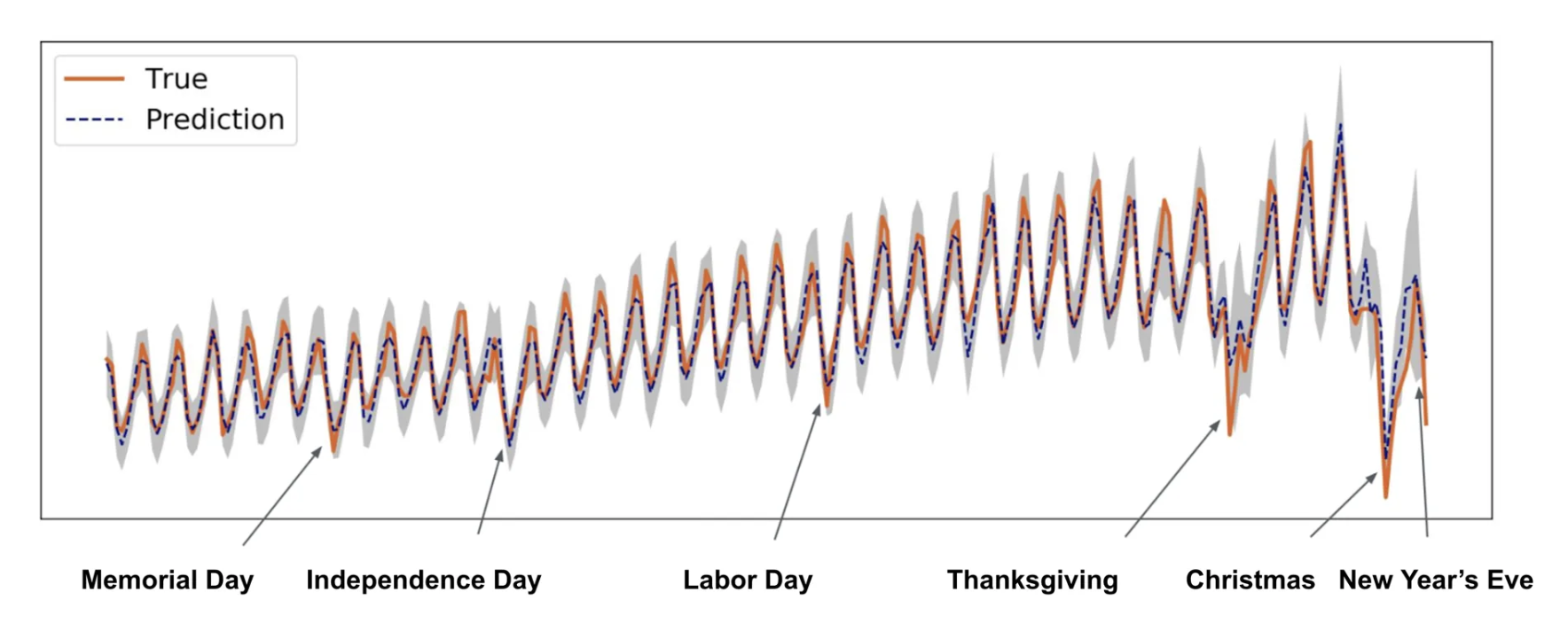
From this image, we see during holiday seasons the upper and lower bounds of the forecasting model get much larger, meaning there's a high level of uncertainty around these events, which makes sense intuitively.
That said, let's replicate this 95% confidence prediction interval for our Bitcoin forecasting ensemble model created in the previous article.
Getting the upper & lower bounds of our prediction interval
In order to get the 95% confidence prediction intervals for our deep learning model, the steps we're going to take include:
- Take the predictions from a number of randomly initialized models (we've already got this from our ensemble model)
- Measure the standard deviation of the predictions
- Multiply the standard deviation by 1.96 (here we're assuming the distribution of our data is Gaussian/Normal—if it is Gaussian this means 95% of the observations fall within 1.96 standard deviations of the mean)
- To get the upper and lower bound prediction intervals, we're going to add and subtract the value obtained in step 3 from the mean/median of the prediction made in step 1
Let's create a function to find the upper and lower bounds of our ensemble model predictions that completes the above steps:
# Find the upper and lower bounds of ensemble predictions
def upper_lower_preds(preds): # 1. Take the predictions from a number of randomly initialized models

  # 2. Measure the standard deviation of the predictions
  std = tf.math.reduce_std(preds, axis=0)

  # 3. Multiply the standard deviation by 1.96
  interval = 1.96 * std

  # 4. Get the prediction interval upper and lower bounds
  preds_mean = tf.reduce_mean(preds, axis=0)
  lower, upper = preds_mean - interval, preds_mean + interval

  return lower, upper
Now we can get the upper and lower bounds of the 95% prediction interval as follows:
lower, upper = get_upper_lower(preds=ensemble_preds)
lower, upper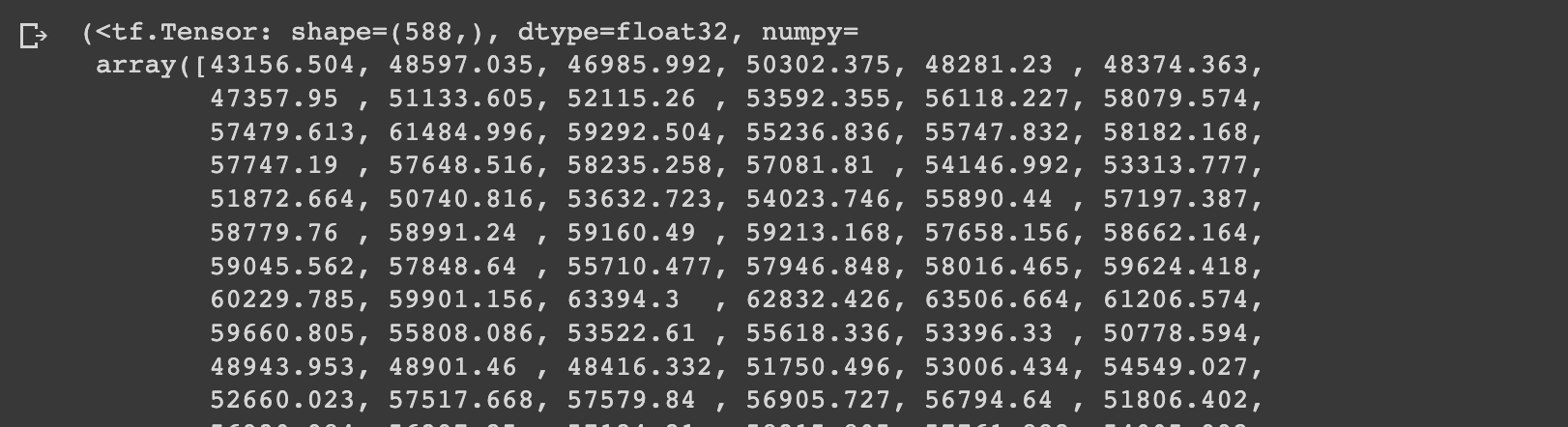
Now that we have the upper and lower bounds, let's plot the prediction intervals of our ensemble model.
Plotting prediction intervals of our ensemble model
In order to plot these prediction intervals, we need to:
- Get the mean and median of our ensemble predictions
- Plot the median of our ensemble predictions along with the prediction intervals
# Get the median/mean values of the ensemble preds
ensemble_median = np.median(ensemble_preds, axis=0)

# Plot the median of the ensemble preds and prediction intervals
offset=500
plt.figure(figsize=(10,7))
plt.plot(X_test.index[offset:], y_test[offset:], "g", label="Test Data")
plt.plot(X_test.index[offset:], ensemble_median[offset:], "k", label="Ensemble Median")
plt.xlabel("Date")
plt.ylabel("BTC Price")
plt.fill_between(X_test.index[offset:],
                 (lower)[offset:],
                 (upper)[offset:], label="Prediction Intervals")
plt.legend(loc="upper left", fontsize=14)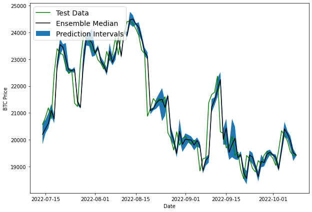
Now we can see we have prediction intervals around our ensemble median. It's also important to note that prediction intervals are also estimates themselves. Also, the prediction intervals have been created with the assumption that our models data follow a normal distribution.
We can also see that it looks like the prediction intervals are lagging behind the ensemble median. This is similar to our naive model that just predicted the previous timestep as the next timestep.
So far we've created several models that are predicting the same results as our baseline model, which indicates that what we're trying to predict is potentially unpredictable...at least with the data we've providing to the model (i.e. previous price data).
This highlights one of the main difficulties with machine learning for time series forecasting, although we'll keep discussing this topic in future articles.
Summary: Prediction Intervals in Forecasting
In this article, we discussed the concept of prediction intervals, also known as uncertainty estimates, which give a range of prediction values with upper and lower bounds.
The use of prediction intervals is common in forecasting due to the uncertainty associated with time series forecasting.
In this case, we replicated a 95% confidence prediction interval for the Bitcoin forecasting ensemble model from our previous article.
Steps to get the upper and lower bounds of the 95% prediction interval include taking predictions from multiple randomly initialized models, measuring the standard deviation of the predictions, multiplying by 1.96, and adding/subtracting from the mean/median of the predictions.
We then created a function to find the upper and lower bounds of the ensemble model predictions and plotted the prediction intervals.
As we saw, the prediction intervals appear to be lagging behind the ensemble median, similar to the naive model that simply predicted the previous timestep as the next timestep, which suggests that the model is not able to accurately predict the future price of Bitcoin with the provided data...
In future articles, we'll discuss more about why forecasting time series data is so challenging and what else we can do to improve our models.


