Mathematics of Machine Learning: Introduction to Probability Theory

In this guide we're going to look at another important concept in machine learning: probability theory.

This is our third article in our Mathematics for Machine Learning series, if you missed the first two  you can check them out below:

• Mathematics of Machine Learning: Introduction to Multivariate Calculus
• Mathematics of Machine Learning: Introduction to Linear Algebra

Probability theory is a broad field of mathematics, so in this article we're just going to focus on several key high-level concepts in the context of machine learning.

This article is based on notes from this course on Mathematical Foundation for Machine Learning and Artificial Intelligence, and is organized as follows:

1. Introduction to Probability Theory
2. Probability Distributions
3. Expectation, Variance, and Covariance
4. Special Random Variables

1. Introduction to Probability Theory

First, why should we care about probability theory?

Probability theory provides a means of quantifying uncertainty and also provides an axiom for deriving new uncertain statements.

Probability theory is very useful artificial intelligence as the laws of probability can tell us how machine learning algorithms should reason.

In short, probability theory gives us the ability to reason in the face of uncertainty.

Where does uncertainty come from?

Uncertainty comes from the inherent stochasticity in the system being modeled.

For example, the financial markets are inherently stochastic and uncertain, so even if we have a perfect model today there's always still uncertainty about tomorrow.

Another source of uncertainty comes from incomplete observability, meaning that we do not or cannot observe all the variables that affect the system.

This connection with this concept and economic models is quite clear, it's simply not possible to know all of the variables affecting a particular market at a given time.

A third source of uncertainty comes from incomplete modeling, in which case we use a model that discards some observed information because the system is too complex.

For example, we still haven't completely modeled the brain yet since it's too complex for our current computational limitations.

Types of Probability

There are a few types of probability, and the most commonly referred to type is frequentist probability.

Frequentist probability simply refers to the frequency of events, for example the chance of rolling two of any particular number with dice is $1/36$.

The second type is bayesian probability, which refers to a belief about the degree of certainty for a particular event. For example, a doctor might say you have a 1% chance of an allergic reaction to something.

To quote Wikipedia:

The Bayesian interpretation of probability can be seen as an extension of propositional logic that enables reasoning with hypotheses

While probability theory is divided into these two categories, we actually treat them the same way in our models.

2. Probability Distributions

In this section we'll discuss random variables and probability distributions for both discrete and continuous variables, as well as special distributions.

Random Variables

As the name suggests, random variable is just a variable that can take on different values randomly.

So the possible values of a variable $x$ could be $x_1, x_2,...x_n$.

A probability distribution specifies how likely each value is to occur.

Random variables can be discrete or continuous variables:

• A discrete random variable has a finite number of states
• A continuous random variable has an infinite number of states and must be associated with a real value

When we have a probability distribution for a discrete random variable it is referred to as a probability mass function.

The three criterion for a discrete random variable to be a probability mass function include:

• The domain of the probability distribution $P$ must be the set of all possible states of $x$
• The probability distribution is between 0 and 1 - $0 \leq P(x) \leq 1$
• The sum of the probabilities is equal to 1, this is known as being normalized - $\sum_{x \epsilon x}P(x) = 1$

Joint Probability Distributions

A joint probability distribution is a probability mass function that acts on multiple variables, so we could have the probability distribution of $x$ and $y$:

$P(x=x, y=y)$ denotes the probability that $x=x$ and $y=y$ simultaneously.

Uniform Distribution

A uniform distribution is a probability distribution where each state of the distribution is equally likely.

This is easy to calculate with discrete values: $P(x=x_i) = \frac{1}{k}$

So what happens when we have a continuous variable?

Probability Density Function

Probability density functions refer to a probability distribution for continuous variables.

This is the type of probability distribution you'll see ubiquitously throughout AI research.

To be a probability density function you need to satisfy 3 criterion:

• The domain of $p$ must be the set of all possible states of $x$
• For continuous variables we can have probabilities greater than 100% $p(x) \geq 0$
• Instead of summation we use an integral to normalize $\int p(x)dx = 1$

Marginal Probability

Marginal probability is the probability distribution over a subset of all the variables.

This comes up in machine learning because we don't always have all the variables, which is one of the sources of uncertainty we mentioned earlier.

With discrete random variables the marginal probability can be foudn with the sum rule, so if we know $P(x,y)$ we can find $P(x)$:

\[P(x= x) = \sum\limits_y P(x = x, y = y)\]

With continuous variables instead of the summation we're going to use the integration over all possible values of $y$:

\[p(x) = \int p(x,y)dy\]

Conditional Probability

Conditional probability is the probability of some event, given that some other event has happened.

Here is the conditional probability that $y = y$ given $x = x$:

\[P(y = y \ | \ x = x) = \frac{P(y=y, x=x)}{P(x=x)}\]

3. Expectation, Variance, and Covariance

Now that we've discussed a few of the introductory concepts of probability theory and probability distributions, let's move on to three important concepts: expectation, variance, and covariance.

Expectation

The expectation of a function $f(x)$ with respect to some probability distribution $P(x)$ is the mean value $f$ takes on when $x$ is drawn from $P$.

What this means is the expectation value is essentially the average of the random variable $x$ with respect to its probability distribution.

The expectation is found in different ways depending on whether or not we have discrete or continuous variables.

For discrete variables we use the summation:

\[\mathbb{E}_{x ~ P}[f(x)] = \sum_x P(x) f(x)\]

For continuous variables we use the integral:

\[\mathbb{E}_{x ~ p}[f(x)] = \int p(x) f(x) dx\]

Variance and Standard Deviation

Here is the formal definition of variance:

Variance ($\sigma^2$) is the expectation of the squared deviation of a random variable from its mean.

In other words, variance measures how far random numbers drawn from a probability distribution $P(x)$ are spread out from their average value.

Here is the formula for variance:

\[Var(f(x)) = \mathbb{E}[(f(x) - \mathbb{E}[f(x)])^2]\]

It's easy to find the standard deviation ($\sigma$) from the variance because it is simply the square root of the variance.

The variance and standard deviation come up frequently in machine learning because we want to understand what kind of distributions our input variables have, for example.

Covariance

From the variance we can find the covariance, which is a measure of how two variables are linearly related to each other.

Here is the equation for covariance:

\[Cov(f(x), g(y)) = \mathbb{E}[f(x)] (g(y) - \mathbb{E}[g(y)])\]

It's important to note that the covariance is affected by scale, so the larger our variables are the larger our covariance will be.

The Covariance Matrix

The covariance matrix will be seen frequently in machine learning, and is defined as follows:

The covariance matrix of a random vector $x$ is an $n$ x $n$ matrix, such that:

\[Cov(x)_{i,j} = Cov(x_i, x_j)\]

Also the diagonal elements of the covariance matrix give us the variance:

\[Cov(x_i, x_i) = Var(x_i)\]

4. Special Random Variables

In this section let's look at a few special random variables that come up frequently in machine learning.

First, what is a special random variable?

A special random variable is a distribution that is commonly found in real life data or in machine learning applications.

The distributions we'll look at include:

• Bernoulli
• Multinoulli
• Gaussian (normal)
• Exponential and Laplace

The Bernoulli Distribution

The Bernoulli distribution is a distribution over a single binary random variable:

\[P(x = 1) = \phi\]

\[P(x = 0) = 1 - \phi\]

We can then expand this to the Multinoulli distribution.

Multinoulli Distribution

This is a distribution over a single discrete variable with $k$ different states. So now instead of just having a binary variable we can have $k$ number of states.

This is also known as a categorial distribution.

The Bernoulli and Multinoulli distribution both model discrete variables where all states are known.

Now let's look at continuous variables.

Gaussian Distribution

The Gaussian distribution is also referred to as the normal distribution, and it is the most common distribution over real numbers:

\[N(x: \mu, \sigma^2) = \sqrt{\frac{1}{2\pi\sigma^2}}exp (-\frac{1}{2\sigma^2}(x - \mu)^2)\]

where:

• $\mu$ is the mean
• $\sigma$ is the standard deviation, and
• $\sigma^2$ is the variance

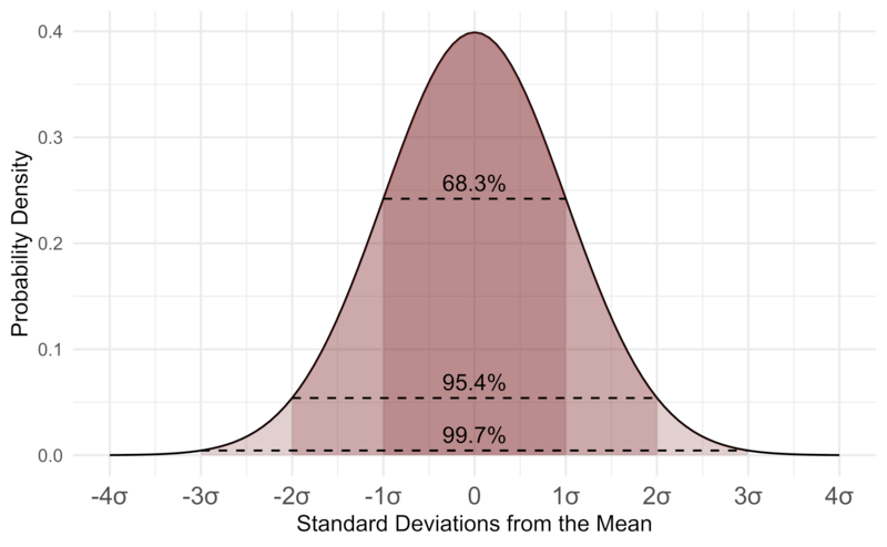
If you've heard of Gaussian distributions before you've probably heard of the 68-95-99.7 rule, which means:

• 68% of the data is contained within +- 1$\sigma$ of the mean
• 95% of the data is contained within +- 2$\sigma$ of the mean
• 99.7% of the data is contained within +- 3$\sigma$ of the mean

Exponential Distribution

Often in machine learning it is beneficial to have a distribution with a sharp point at $x = 0$, which is what the exponential distribution gives us:

\[p(x; \lambda) = \lambda 1_{x \geq 0} exp(-\lambda x)\]

Laplace Distribution

The Laplace distribution is the same as the exponential distribution except that the sharp point doesn't have to be at the point $x = 0$, instead it can be at a point $x = \mu$:

\[Laplace \ (x; \mu, \gamma) = \frac{1}{2\mu}exp (-\frac{|x - \mu|}{\gamma})\]

The exponential and Laplace distribution don't occur as often in nature as the Gaussian distribution, but do come up quite often in machine learning.

Summary: Machine Learning & Probability Theory

In this article we introduced another important concept in the field of mathematics for machine learning: probability theory.

Probability theory is crucial to machine learning because the laws of probability can tell our algorithms how they should reason in the face of uncertainty.

In terms of uncertainty, we saw that it can come from a few different sources including:

• Inherent stochasticity
• Incomplete observability
• Incomplete modeling

We also saw that there are two types of probabilities: frequentist and Bayesian. Frequentist probability deals with the frequency of events, while Bayesian refers to the degree of belief about an event.

We then looked at a few different probability distributions, including:

• Random variables
• Joint probability distribution
• Uniform distribution
• Probability density function
• Marginal probability
• Conditional probability

Next, we looked at three important concepts in probability theory: expectation, variance, and covariance.

Finally, we introduced a few special random variables that come up frequently in machine learning, including:

• Bernoulli distribution
• Multinoulli distribution
• Gaussian (normal) distribution
• Exponential and Laplace distribution

Of course, there is much more to learn about each of these topics, but the goal of our guides on the Mathematics of Machine Learning is to provide an overview of the most important concepts of probability theory that come up in machine learning.

Resources:

• Mathematical Foundation for Machine Learning and Artificial Intelligence