Quantum Programming with the D-Wave Quantum Annealer

In our last article on quantum programming with Google Cirq we finished off by creating a quantum Fourier transform circuit.

In this article we're going to build off of this and program the D-Wave quantum annealer to solve several real-world problems.

This article is based on this quantum computing course, and is organized as follows:

1. What is Quantum Annealing?
2. Installing the D-Wave Ocean SDK
3. What is a Graph Problem?
4. Solving the Graph Problem with a QPU
5. What is Constraint Analysis?
6. What are Binary Quadratic Models?
7. Reading Minimum Energy Levels on a QPU
8. Summary: Quantum Programming with D-Wave

1. What is Quantum Annealing?

Here's the definition of quantum annealing from Wikipedia:

Quantum annealing (QA) is a metaheuristic for finding the global minimum of a given objective function over a given set of candidate solutions (candidate states), by a process using quantum fluctuations.

In other words, the main task of a quantum annealer is to find the minimum energy distribution of a given space.

Here's how quantum annealing works with D-Wave:

The quantum bits—also known as qubits—are the lowest energy states of the superconducting loops that make up the D-Wave QPU.

Let's now look at how we can program a D-Wave QPU.

2. Quantum Programming with D-Wave Leap

For this article we're going to make use D-Wave Leap, which gives you access to the D-Wave 2000Q quantum computer for 1 minute of QPU each month.

Doesn't sound like a lot but with a QPU that's more than enough to get started, and as the company mentions "is enough to run between 400 and 4000 problems".

After creating an account we need to install the D-Wave Ocean Software Development Kit, which is:

a suite of tools D-Wave Systems provides on the D-Wave GitHub repository for solving hard problems with quantum computers.

To get started we're going to pip install dwave-ocean-sdk.

After installing the dependancies we need to configure a solver, as:

Most Ocean tools solve problems on a solver, which is a compute resources such as a D-Wave system or CPU, and might require that you configure a default solver.

To do this we're going to use the command dwave config create.

We then need to specify a configuration file path, if you don't want to change it just press enter and create the default path.

Next we going into the production profile, or prod, and we can skip the API endpoint URL.

After this we need to enter our authentication token from the Leap dashboard and enter it.

We want to solve our problem on a QPU so next we enter QPU into the command line.

We can use the default solver and now our configuration is saved.

Now, with the use of the Ocean SDK this will be executed with the profile we just saved with our API token.

Now let's start programming a graph problem that can be solved with a QPU.

3. What is a Graph Problem?

Let's now look at a problem that is well suited for a quantum computer: a graph problem.

To understand this let's look at an example.

Let's say that we are a city planner and want to set up traffic camera's throughout the city.

So the task is to cover every car that drives through the city, and let's assume that installing the cameras is quite expensive so we have two conditions:

• We need to figure out a way to use the minimum number of cameras
• We need to cover every car that is driving from one place to another

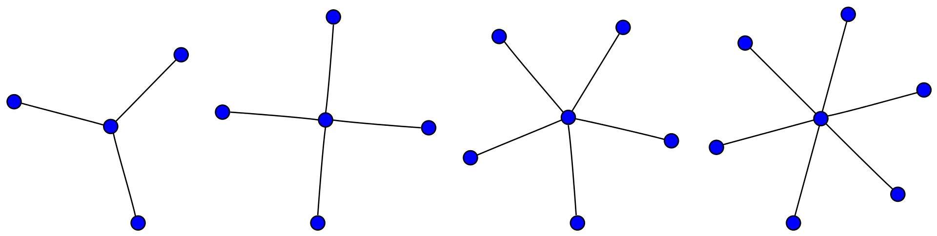
Let's start with a well known graph: a star graph.

In this graph we have a center, which we'll call $K$, and then we have 4 nodes, $A$, $B$, $C$, and $D$.

In this case if we position the camera at location $K$ if a car want's to drive from $K$ to any location it is covered.

In the image below we can see an example of a star graph with 3, 4, 5, and 6 nodes:

So the goal with the D-Wave QPU will be to get the location of $K$.

If we were using a classical computer the most basic way to solve this would be to calculate the number of nodes, 5 in this case, and then calculate the number of possible journeys between each node.

We would then look at each journey and determine if we have a camera covering it or not.

This would be fine for a classical computer to solve with only 5 nodes, but as soon as we get to 100+, or 1000+, which is the case with real cities, calculating the number of possible options becomes non-trivial.

Enter the QPU.

This problem is well suited for a quantum computer because it can consider the entire solution set at once.  Coming back to the quantum annealer, in this example we want to find the minimum energy to solve this problem.

So the D-Wave quantum annealer will scan through the entire solution space and return an optimal solution given our 2 constraints - for each car to be covered by a camera, and with the minimum number of cameras.

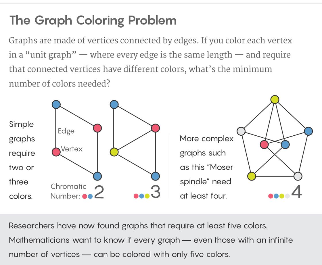
If you want to read more about the graph problem check out this article on the Graph Coloring Problem:

4. Solving the Graph Problem with a QPU

To solve the graph problem let's start by creating an interface with our star graph.

To do this we're going to use the NetworkX, which is:

a Python package for the creation, manipulation, and study of the structure, dynamics, and functions of complex networks.

First we import NetworkX and then we'll define a star graph with 5 nodes.

Then we're going to solve the graph problem on a QPU, and to do this we need 2 main components:

• A sampler
• A composite

These components together convert the problem into a quadratic model, which is then transferred onto the D-Wave quantum computer.

We'll get into quadratic models later, but for now it's a way to convert a problem into a language the quantum computer can understand.

To solve the problem on a QPU we need to import the sampler and composite from the D-Wave Ocean SDK.

Now we need to declare a sampler, which is equal to EmbeddingComposite(), and inside it we pass in the DWaveSampler().

We're now ready to solve the graph problem with the sampler we just created.

To do this we're going to import dwave_networx as dnx and thenprint(dnx.min_vertex_cover()) and then we pass in the graph s5 and the sampler.

import networkx as nx
import dwave_networkx as dnx
from dwave.system.samplers import DWaveSampler
from dwave.system.composites import EmbeddingComposite

# create a graph
s5 = nx.star_graph(50)

# solve on a QPU
sampler = EmbeddingComposite(DWaveSampler())
print(dnx.min_vertex_cover(s5, sampler))

After we run this we get a [0] in the command line, which means we have the central node, or the answer to the problem.

Now that we've looked at a graph problem, let's move on to a new type of problem: constraint analysis.

5. What is Constraint Analysis?

Constraint analysis is an important concept to cover in quantum computing.

The example we're going to look at with D-Wave solves a binary constraint satisfaction problem (CSP):

CSPs require that all a problem’s variables be assigned values that result in the satisfying of all constraints.

In this example we have 4 constraints for scheduling meetings.

Based on these constraints we're going to use a QPU to find the best possible combination of meetings that satisfies all of the constraints.

The first step to solve this with D-Wave is to express the problem as a binary quadratic model.

So we're going to define 4 variables as either a 0 or a 1: time, location, length, and mandatory.

Since we have 4 binary variables there are $2^4$ or $64$ possible meeting arrangements.

In this example we can create a table that outlines the situations that satisfy all 4 constraints.

This is easy to do with 4 variables, but is very computationally expensive - if we have 20 variables we'd have to check 1,048,576 entries.

This makes a good problem for a quantum computer to solve, so to solve this we can use D-Waves Binary CSP, which is a:

library to construct a binary quadratic model from a constraint satisfaction problem with small constraints over binary variables.

For this example we need to define a function that returns True when all the constraints are met, but first let's review another important concept.

6. What are Binary Quadratic Models?

Binary quadratic models (BQM) are another important concept in quantum computing.

Binary quadtraic models are particularly important because they're the only language that the current D-Wave quantum computers understand.

So whenever we want to submit a problem to a QPU we have to convert it to a binary quantratic model.

Let's breifly review the mathematics of a binary quadratic model.

From Wikipedia we get the definition:

a binary quadratic form is a quadratic homogeneous polynomial in two variables

We also get the equation:

\[q(x, y) = ax^2 + bxy + cy^2\]

So we have a function $q$ which is a function of two variables $x$ and $y$, and $a$, $b$, and $c$ are the coefficients.

We can see the right side of the equation is a quadratic equation because we have $x^2$ and $y^2$.

What the D-Wave quantum computer gives us from this binary quadratic equation is the optimal value of $a$, $b$, and $c$, and based on these values we can get the desired output.

Coming back to our constraint scheduling problem, we mentioned that this task is dependant on 4 varaibles: time, location, length, and mandatory.

Using the dwavebinarycsp library we can express these constraints in a binary quadratic model by just defining a function that evaluates True when the constraints are met.

Defining the Binary Quadratic Model

Let's now define a method called scheduling and then we'll convert this to a binary quadratic model.

The code below is a function that returns True when all the constraints are met:

def scheduling(time, location, length, mandatory):
    if time:                                 # Business hours
        return (location and mandatory)      # In office and mandatory participation
    else:                                    # Outside business hours
        return ((not location) and length)   # Teleconference for a short duration

Now let's generate a binary quadratic model based on this with dwavebinarycsp.

First define our constraints csp, and then we generate a binary quadractic model bqm:

import dwavebinarycsp

csp = dwavebinarycsp.ConstraintSatisfactionProblem(dwavebinarycsp.BINARY)
csp.add_constraint(scheduling,['time', 'location', 'length',])

bqm = dwavebinarycsp.stitch(csp)

7. Reading Minimum Energy Levels on a QPU

Now that we have created a binary quadratic model let's run the problem on the D-Wave QPU.

The main challenge now is processing the data on a QPU and then displaying it a human-readable format.

Just like we did in the graph project we need to import a sampler DWaveSampler and a composite EmbeddingComposite

We then need to specify:

sampler = EmbeddingComposite(DWaveSampler())

We then need to get a response from the QPU:

response = sampler.sample(bqm, num_reads = 5000)

By reading the QPU 5000 times this reduces the chance that we are getting a sub-optimal output.

We then need to set the total to 0 and then loop through the response data:

total = 0

for sample, energy, occurences in response.data(['sample', 'energy', 'num_occurences']):
    total = total + occurrences
    if energy == min_energy:
        time = 'business hours' if sample['time'] else 'evenings'
        location = 'office' if sample['location'] else 'home'
        length = 'short' if sample['length'] else 'long'
        mandatory = 'mandatory' if sample['mandatory'] else 'optional'
        print('{}: During {} at {}, you can schedule a {} meeting this is {}'.format(occurences, time, location, length, mandatory))

Now we have converted the minimum energy value in a way that is human-readable, and then we need to print the output generated from the analysis.

The last thing we need to do is define the min_energy:

min_energy = next(response.data(['energy']))[0]

Let's run the full code on the D-Wave Leap QPU:

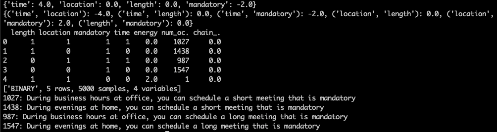
We now have a list of options for scheduling meetings that satisfy all of the problem's constraints.

8. Summary: Quantum Programming with D-Wave

In this article we looked at how to program a quantum computer with D-Wave Systems.

We first discussed what quantum annealing is and how D-Wave uses it to find the minimum  energy distribution of a given space.

We then looked at how we can use this to solve two types of problems: a graph problem, and a contraint analysis problem.

We then discussed binary quadratic models, which are the language that the current D-Wave quantum computers understand.

Finally we ran the model on a QPU with D-Wave Leap to solve a constraint analysis problem.

Resources:

• Quantum Computing: Theory to Simulation and Programming