
In this article we'll review the fundamental mathematics required to analyze and solve quantum computing problems. The article will assume you have some knowledge of quantum computing, if not you can check out these resources:
- What is Quantum Computing? Key Concepts & Industry Use Cases
- Quantum Machine Learning: Introduction to Quantum Systems
- Quantum Machine Learning: Introduction to Quantum Learning Algorithms
- Quantum Machine Learning: Introduction to Quantum Computation
- Introduction to Quantum Programming with Google Cirq
- Quantum Programming with the D-Wave Quantum Annealer
- Introduction to Quantum Programming with Qiskit
This article is based on this course on Advanced Math for Quantum Computing, and will first provide a brief review of quantum computing and then discuss several key mathematical concepts.
1. Quantum Computing Review
Let's briefly review key concepts of quantum computing.
A qubit is a quantum bit that can be 0, 1, or in superposition between 0 and 1.
The state of a qubit can be represented by the following matrices:
$$0 = |0\rangle = \begin{bmatrix}1 \\0\end{bmatrix}$$
$$1 = |1\rangle = \begin{bmatrix}0 \\1\end{bmatrix}$$
A state vector is a column matrix that represents a quantum state.
Keep in mind that $|0\rangle$ and $|1\rangle$ are names of matrices for the qubit state they represent, they are not actually numeric values.
The numbers inside a state vector are the square root of probabilities. They are complex values that are used in qubit state computations.
The notation for $|0\rangle$ and $|1\rangle$ is called a "ket", which is the matrix itself with no changes.
The "bra" operation complements the "ket" and is notated with a left angle bracket and vertical bar as follows:
$$\langle 0| = 0^+$$
$$\langle 1| = 1^+$$
The bra operation is the same as the adjoint operation, which is represented by the $^+$. The adjoint operation is the transpose of the complex conjugate.
Two special matrices whose properties are defined by their adjoints include:
- Unitary: if the adjoint of a matrix is the same as its inverse, it is said to be unitary.
$$U^+ = U^{-1}$$
- Hermitian: if the adjoint of a matrix is the matrix itself, it is said to be Hermitian.
$$H^+ = H$$
Finally, eigenvectors and eigenvalues are important concepts, here is a quick review:
Given a matrix $A$, you might be able to compute a vector $V$ such that when $A$ is multiplied by $V$ the result is the same as multiplying a scalar $e$ by $V$:
$$AV = eV$$
where:
- $V$ is eigenvector of $A$
- $e$ is the eigenvalue of A corresponding to vector $V$
Each different matrix $A$ will have a different set of eigenvectors and eigenvalues.
2. Key Concepts: Mathematics of Quantum Computing
In this section we'll review several key mathematical techniques of quantum computing, including:
- Probability of Measurement
- Orthonormality
- Orthonormality in Bracket Notation
- Basis Vectors
- Degrees of Freedom
- Degrees of Freedom of a Single Qubit
- Global & Relative Phase
- Bloch Sphere
- Entanglement & Degrees of Freedom
- Testing for Entanglement
Probability of Measurement
A quantum state is represented by a column matrix, which is also called a vector.
If we have a vector $S$ to represent the state of the system and we have another vector $A$ to represent the measurement apparatus—meaning the system $S$ is measured by the apparatus $A$.
In an idealized measurement, the system will report that it is aligned with the apparatus or not. This means that the result of measurement is either "aligned" or "not aligned".
The equation for a probability of measurement is aligned is as follows:
$$|A|S|^2 = (|<A|x|S>|)^2 = |A^+S|^2 = |<S|A>|^2 = (|<S|x|A>|)^2 = |S^+A|^2$$
Recall that the squared magnitude of $|<S|A>|$ is the same as the squared magnitude of $|<A|S>|$.
Orthonormality
The vectors $\begin{bmatrix}1 \\0\end{bmatrix}$ and $\begin{bmatrix}0 \\1\end{bmatrix}$ are orthogonal to each other.
If an apparatus is in $\begin{bmatrix}0 \\1\end{bmatrix}$ and a qubit state is $\begin{bmatrix}1 \\0\end{bmatrix}$ the probality of a measurement being "aligned" is 0:
$$|<S|A>|^2 = 0$$
If the apparatus is $\begin{bmatrix}1 \\0\end{bmatrix}$ and the qubit state is $\begin{bmatrix}1 \\0\end{bmatrix}$, again the probability of being "aligned" is 0.
Recall that the magnitude of a vector $\begin{bmatrix}a \\b\end{bmatrix}$ is 1:
$$\sqrt{|a|^2 + |b|^2 = 1}$$
When the magnitude is 1, we call the vector a unit vector. When the magnitude is 1, the squared magnitude is also 1.
If a vector is both orthogonal and unit vectors, they are orthonormal. The notation for orthonormality is as follows:
- $||$ the vertical bars denote magnitude
- $^*$ superscript star indicates complex conjugation
For example, given two vectors $\begin{bmatrix}a \\b\end{bmatrix}$ and $\begin{bmatrix}c \\d\end{bmatrix}$, all of which may be complex numbers, the following conditions must be met for the two vectors to be orthnormal:
$$|a|^2 + |b^2| = 1$$
$$|c|^2 + |d^2| = 1$$
$$[a* b*] \begin{bmatrix}c \\d\end{bmatrix} = 0$$
Orthonormal vectors are important because any vector can be written as a linear combination of orthonormal vectors.
Orthonormality in Bracket Notation
Here is a review of orthonormality in bracket notation:
- X and Y are unit vectors, meaning the magnitude of X and Y is 1:
$| |X> | = 1$ and $| |Y> | = 1$
- Bracket $X$ and $Y$ is 0:
$<X|Y> = 0$
- The bracket of any unit vector with itself is 1:
$<X|X> = 1$ and $<Y|Y> = 1$
A set of vectors that are orthonormal to each other is called an orthonormal set. If we have an othornomal set of vectors:
- Bracket of a vector with itself is 1
- Bracket of a vector with any other vector in the set is 0
$<V_i|V_j> = 1$, when $i = j$
$<V_i|V_j> = 0$, when $i \neq j$
The maximum number of elements in an orthonormal set is equal to the number of vector dimensions. In other words, for $n$ dimensional vectors, an orthonormal set can have a maximum of $n$ vectors.
Basis Vectors
If we have a two coordinate space of $x$ and $y$ axis...
We also define a unit vector $\hat{x}$ along the $x$ axis and unit vector $\hat{y}$ along the $y$ axis. This means that any point in the coordinate space can be described as:
$$a\hat{x} + b\hat{y}$$
This means that any vector from the origin point can be written as a linear combination of the unit vectors $\hat{x}$ and $\hat{y}$.
$\hat{x}$ and $\hat{y}$ are also orthogonal to each other.
The point is, if any two unit vectors are orthogonal we can write any vector as a linear combination of the two vectors.
Thus, we can use any pair of orthogonal unit vectors instead of $\hat{x}$ and $\hat{y}$.
In the context of quantum computing, we first state a problem by choosing a set of orthonormal vectors.
We then express all other vectors in terms in terms of the orthonormal vectors we choose, which are referred to as basis vectors.
Degrees of Freedom
Suppose we have a physical system and the state of it can be described by real numbers.
The minimum number of states required to describe the system is the degrees of freedom of the system. This concept applies to both quantum and classical systems.
A simple classical system is temperature, which can be represented as a single real number. There are an infinite number of states that can be represented by the real number for temperature.
If we have a system with two degrees of freedom, there is also an infinite number of states—except this is a larger set than the single degree of freedom.
The point is that larger the number of degrees of freedom result in larger infinite possible states of a system.
As we'll discuss below, degrees of freedom is a critical concept for understanding entanglement between qubits.
Degrees of Freedom of a Single Qubit
A single qubit state is represented by a column matrix with two complex elements, each of which has two real numbers:
$$\begin{bmatrix}a+ib \\c+id\end{bmatrix}$$
where a, b, c, & d are real numbers.
There are two constraints on a single qubit system:
- The requirement that state vectors are unit vectors since the sum of probabilities must be one:
$$a^2 + b^2 + c^2 + d^2 = 1$$
- The other constraint is from the physical state of quantum systems, which says that $|S\rangle$ and $e^{i\theta} | S\rangle$ are the same state.
The number of degrees of freedom of a single qubit state is 4 real parameters - 2 constraints, so it is 2.
Next we will discuss how entanglement occurs in system with more than 1 qubit.
Global & Relative Phase
As mentioned, the global phase does not affect physical behaviour. Global phase, however, should not be confused with relative phase.
If we have a state vector $\begin{bmatrix}a\\b\end{bmatrix}$ that are complex numbers.
The relative phase between $a$ and $b$ can be described as follows:
$$e^{i\phi} = \frac{a |b|}{|a| b}$$
- where $\phi$ is the relative phase in the equation
Unlike the global phase, the relative phase is physically important. In other words, when doing quantum math you can't just substitute one vector with another because it is physically equivalent.
Bloch Sphere
Earlier, we defined the standard basis vectors as:
$$|0\rangle = \begin{bmatrix}1\\0\end{bmatrix}$$
$$|1\rangle = \begin{bmatrix}0\\1\end{bmatrix}$$
There is also the Hadamard basis, which uses the vectors ket-plus and ket-minus:
$$|+\rangle = \frac{1}{\sqrt2}(|0\rangle + |1\rangle)$$
$$|-\rangle = \frac{1}{\sqrt2}(|0\rangle - |1\rangle)$$
The ket-plus and ket-minus are simply the conventional name of these vectors.
In order to represent state vectors visually we can use a Bloch sphere.
One point of confusion is that we previously computed state vectors for spin along the X, Y, and Z directions. When dealing with a Bloch sphere, however, do not try and associate a direction.
The Bloch sphere is simply a way to visually represent state vectors—its three axes do not always correspond to cartesian coordinates i.e. X, Y, and Z in physical space.
Given two angles $\theta$ and $\phi$, we can map those angles to plot the state vector on the surface of the Bloch sphere as follows:
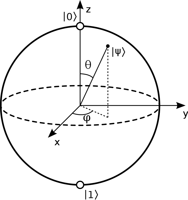
Opposite points on the Bloch sphere represent state vectors that are orthogonal.
Recall that the state vector of a qubit has 2 degrees of freedom, which indicates that a state vector can only be mapped to a point on the surface of the Bloch sphere.
Entanglement & Degrees of Freedom
Revisiting the degrees of freedom concept, suppose we have 2 systems each with 2 degrees of freedom.
If we combine the two systems, the combination would have 4 degrees of freedom.
System AB is defined by $(x_a, y_b, x_b, y_b)$
In the case of quantum physics, if we combine two particles and "glue" them together, this property would add more degrees of freedom to the combined system. In other words, there would be 5 or more degrees of freedom.
When we combine two single qubit systems, each qubit has 2 degrees of freedom.
In this case, there are 4 complex numbers, or 8 real parameters, 2 constraints (sum of probabilities = 1, global phase is irrelevant).
This means there are 8 - 2 = 6 degrees of freedom, and this is how entanglement can be explained in terms of degrees of freedom
Testing for Entanglement
A tensor product $A\otimes B$ is always an unentangled state, which gives us a test for entanglement.
If a state vector of a multi-qubit system can be expressed as a tensor product of single-qubit state, then it is not entangled.
On the other hand, the basis vectors used don't matter in determining in a state is entangled or not.
Summary: Mathematics of Quantum Computing
In this article we reviewed key mathematical concepts of quantum computing, including:
- Probability of Measurement
- Orthonormality
- Orthonormality in Bracket Notation
- Basis Vectors
- Degrees of Freedom
- Degrees of Freedom of a Single Qubit
- Global & Relative Phase
- Bloch Sphere
- Entanglement & Degrees of Freedom
- Testing for Entanglement


