

Let’s talk about the nature of learning. We aren't born knowing much, but over the course of our lives, we develop an understanding of the world through interaction.
Through this trial and error approach to interacting with the world, we develop an understanding of how the world responds to our actions, or cause and effect.
In this article, we’ll take a scientific stab at understanding at how this learning process through trial and error happens. To do this, we’ll use a computational approach called: reinforcement learning.
In order to gain an understanding of reinforcement learning, we’ll simplify things by using environments with well-defined rules and dynamics before getting into the endlessly complex real world.
We’ll look at several reinforcement learning algorithms that solve the learning-by-interaction problem, and look at the strengths and weaknesses of each. In particular, we'll discuss:
- Applications of Reinforcement Learning
- Learning from Action: the RL Approach
- Review of Supervised Learning
- Review of Unsupervised Learning
- The Reinforcement Learning Problem
- Important RL Concepts
- Introduction to OpenAI Gym
- The Bellman Equation and Reinforcement Learning
- Markov Decision Processes and Reinforcement Learning
- The Exploration-Exploitation Dilemma
- Summary: What is Reinforcement Learning?
Let's start with the fun part: applications of reinforcement learning.
Stay up to date with AI
1. Applications of Reinforcement Learning
There are many exciting applications of reinforcement learning that are making headlines daily. We're going to look at a few applications including:
- Board games
- Video games
- Self-driving cars
- Robotics
Board games
One of the most famous examples of reinforcement learning in action is the DeepMind AlphaGo victory over Lee Sedol in the game of Go.
The reason that this victory in the game of Go is that it has more than 300 times the number of plays as chess, and...
It’s said that there more configurations in the game of Go than there are atoms in the observable universe.
To learn more about this, I highly recommend the AlphaGo movie.

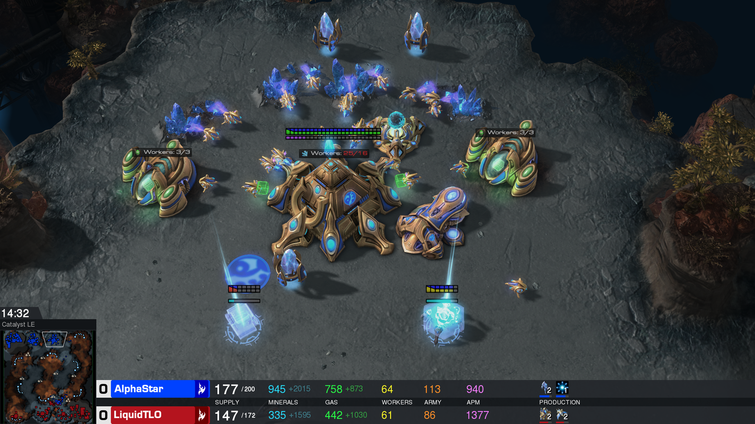
Video Games
More recently, DeepMind used reinforcement learning to create AlphaStar, the first Artificial Intelligence to defeat a top professional player.
You can read more about that here on their blog.
Robotics
Another widely used application of reinforcement learning is in the field of robotics.
The idea is that we can give robots this learn-by-interaction approach for a robot to test out walking, or moving an arm, for it to see what works and what doesn’t work. We then create an algorithm to help the robot learn from this experience it gained.
Self-driving cars
Reinforcement learning has successfully been applied to self-driving cars, airplanes, and ships.
There are many other applications of reinforcement learning, and here are several resources on each industry:
- Biology - you can read this paper on the topic
- Inventory Management - you can read this paper on the topic
- Telecommunications - Check out this paper on RL for low-power wireless communication.
- Finance - check out this Github project and this article
2. Learning from Action: the RL Approach
Now let's look at how this learning from interaction actually happens.
In the field of reinforcement learning, the learner, or decision maker is referred to as the agent.
When an agent first enters an environment, it has no idea how anything works. An agent has a set of actions that it can take, but it has no idea how these actions will affect the environment.
Let’s say for the first action the agent just picks one at random.
After an action is taken (for simplicity purposes), there is either a reward or a punishment from that environment.
Let’s also assume that the sole purpose of the agent is to maximize reward.
While it may seem easy to simply learn from the environment, there are a few challenges.
One of them is that the agent has an exploration-exploitation dilemma:
- Exploration means the agent is exploring potential hypotheses for how to choose actions, which inevitably will lead to some negative reward from the environment.
- Exploitation means how the agent exploits the limited knowledge about what it has already learned.
So the question here is how should an agent balance these two competing requirements to achieve optimal results?
The answer to this remains an active field of research.
Before getting into the topic of RL algorithms, let's first review the three main branches of machine learning: supervised, unsupervised, and reinforcement learning.
3. Review of Supervised Learning
The majority of introductory machine learning algorithms start with supervised learning.
In the machine learning pipeline, the first step is typically to collect a dataset, which comes in a variety of file formats.
In a supervised learning problem, we're trying to predict a value that already exists, this is known as the label, the target variable, or the dependent variable. The rest of the features are known as independent variables.
The thing to remember about supervised learning is that the data we'd use to train our model already contains the desired response—that is, it contains a dependent variable.
Supervised learning is good for these types of problems:
- Classification: Sorting items into classes, such as cats and dogs
- Regression: Identifying real values such as dollars, weights, etc.
Most data, however, doesn't have clean labels for us to use, but we still want to derive some insights from it.
This is where unsupervised learning comes in.
4. Review of Unsupervised Learning
The first step in unsupervised learning is to provide the machine learning algorithm with uncategorized, unlabelled data to see what patterns it can find.
We then observe and learn from the patterns that the machine identifies.
This allows us to visualize groups of data points that we wouldn't otherwise know of.
Unsupervised Learning is good for these types of problems:
- Clustering: Identifying similarities in groups
- Anomaly detection: Identifying abnormalities in our data
Unsupervised learning algorithms are often used to preprocess data, for example during the exploratory data analysis stage it can be used to cluster groups of data.
Both supervised and unsupervised learning algorithms are incredibly useful tools to recognize complex patterns in data.
But what if, for example, our goal is to optimize the product delivery in a supply chain. In particular, we want to predict the most optimal delivery route given all other factors such as weather, transportation schedules, etc.
This is a very dynamic problem space.
So what is the best learning algorithm to use?
Well, we need a learning system that is highly adaptive to changes.
We also don't have a pre-existing dataset to learn from, the algorithm needs to learn in real-time.
This problem also introduces a new dimension: time.
This is the task that reinforcement learning attempts to solve.
5. The Reinforcement Learning Problem
The problem that we are trying to solve with Reinforcement Learning is somewhere in between supervised and unsupervised learning.
In the RL framework, an agent learns to interact with its environment.
In the environment we assume that time passes in discrete time-steps.
As the agent takes an action, we then get time-delayed labels that are sparse.
From these labels, which we can call rewards, the agent gets a new observation and then must select another action, at the next time step.
The observation is called a state.
It is essentially a feedback loop of state -> action -> reward.
The goal of the agent is (assumed) to be to maximize expected cumulative reward.
The agent seeks to find a set of actions for which the cumulative reward is expected to be high.
The agent can only only accomplish its goal by interacting with the environment.
Through interaction the agent can learn the rules of the environment, and then after training can choose a set of actions to accomplish its goal.
It is the powerful combination of pattern-recognition networks and real-time environment based learning frameworks called deep reinforcement learning that makes this such an exciting area of research.
6. Important RL Concepts
Now let's discuss several key concepts in the field of reinforcement learning.
Episodic vs. Continuing Tasks
Many of the examples used in this article will have a well defined endpoint, for example, video games have a clear end when the agent wins or loses.
These are called episodic tasks, or tasks that end at some time step $T$.
Each sequence from the initial state and action to the end is called an episode.
The agent can then review of the cumulative reward it received for that episode, learn from this new information, and adjust its parameters accordingly.
Over time, the agent should be able to pick a strategy where the total reward is quite high.
We'll also look at continuous tasks, or tasks where the interaction continues without an end-point.
An example of continuous tasks in the real-world are trading in the financial markets, since the markets never really have an end date.
In this case, the agent must learn how to operate in its environment and simultaneously maximize it's expected reward.
Understanding Rewards
Whether the goal is to win a game of Go, driving a self-driving car, or a robot learning how to walk - the RL problem can be addressed with the same theoretical framework.
The question is then...
How can we define the concept of reward for any goal that our agent has?
Remember that the reward hypothesis is that...
All goals can be framed as the maximization of expected cumulative reward.
6. Introduction to OpenAI Gym
In order to train our agents in different environments, we'll make use of the open-source OpenAI Gym, which is a...
toolkit for developing and comparing reinforcement learning algorithms. It supports teaching agents everything from walking to playing games like Pong or Pinball.
If you want to install gym on your computer, you can find the Github here.
We're first going to spend a bit of time developing the theory behind reinforcement learning before getting into OpenAI Gym...just something to look forward to.

7. The Bellman Equation and Reinforcement Learning
One of the most fundamental and important mathematical formulas in reinforcement learning is the Bellman Equation.
The here goal is to provide an intuitive understanding of the concepts in order to become a practitioner of reinforcement learning, without needing a PhD in math.
The key to developing this understanding is to first get comfortable with the nomenclature of the subject.
Dr. Richard Bellman
The roots of reinforcement learning actually go back to Dr. Richard Bellman in 1954. He is known as the Father of Dynamic Programming.
The Bellman equation is presented in his 1954 paper "The Theory of Dynamic Programming".
Dynamic Programming
Dynamic programming is a class of algorithms that seek to simplify complex problems by breaking them up into sub-problems, and solving the sub-problems recursively - meaning a function calls itself repeatedly until it comes up with the right solution.
The Goal of Reinforcement Learning
To review, what are we actually trying to accomplish with reinforcement learning?
Given the current state we are in, the goal of reinforcement learning is to choose the optimal action which will maximize the long-term expected reward provided by the environment.
What Question Does the Bellman Equation Solve?
The question this equation solves is:
Given the state an agent is in, assuming it take the best possible action now and at each subsequent step, what long-term reward can it expect?
In other words, what is the value of the state?
Of course, not all states are of equal value.
The Bellman Equation helps us evaluate the expected reward relative to the advantage or disadvantage of each state.
Bellman Equation for Deterministic Environments
Below is the Bellman equation for deterministic environments:
$$V(s) = max_a(R(s,a) + \gamma V(s'))$$
The value of a given state is equal to max action, which means of all the available actions in the state we're in, we pick the one that maximizes value.
We take the reward of the optimal action \(a\) in state \(s\) and add a multiplier of gamma, which is the discount factor which diminishes our reward over time.
Each time we take an action we get back the next state: \(s'\)
This is where dynamic programming comes in, since it is recursive we take \(s'\) and put it back into the value function \(V(s)\).
We continue that until we get the terminal state and we know the value of the state we're in, assuming we choose the optimal action.
The catch is that at each step we have to know what the optimal action is which will maximize the expected long term rewards.
In the days before the Deep Learning Revolution, this was done by trying out all actions in a huge search tree. The problem with this is that the brute force approach can be difficult when faced with complex tasks, such as playing video games based off of raw pixels.
This is where deep neural networks changed everything—instead of trying every possible action in every possible state, the network can simply estimate the value of the state and intelligently guess which action will maximize it.
Important Points About Gamma
An important part to understand is why the discount factor, gamma \(\gamma\), is so important.
If \(\gamma\) is 1, meaning there is no discounting, we have the problem of sparse rewards.
Every other state that isn't a reward or punishment state is 0, so with no discount all the states end up with equal values of 1 and don't teach the model anything.
Key points to remember include:
- It is important to tune this hyperparameter to get optimum results.
- Successful values often range from 0.9 to 0.99.
- A lower value encourages short-term thinking
- A higher value emphasizes long-term rewards
Also keep in mind that this equation assumes that we're choosing the optimal value in each state, which we haven't covered yet in this article.
In other posts, we will discuss the various techniques to estimate the optimal actions, given imperfect information. All of these techniques, however, are built on top of concepts from the Bellman Equation.
8. Markov Decision Processes
An important framework for representing the reinforcement learning problem of an AI agent learning in an environment is called a Markov Decision Process (MDP).
This framework allows actions (i.e. choices) and rewards.
A Markov Decision Process is defined by 5 components:
- A set of possible states
- An initial state
- A set of actions
- A transition model
- A reward function
Since we have a reward function we can conclude that some states are more desirable than others.
The problem is that the agent has to maximize the reward by avoiding states that return negative values and choosing the one which returns positive values.
The solution is to find a policy that selects the action with the highest reward.
An agent can try many different policies, although the one we are looking for is the optimal policy, which gives us the best utility.
Reinforcement learning deals with an agent that interacts with its environment in the setting of sequential decision making.
It does this by trying to choose optimal actions (among many possible actions) at each step of the process.
We refer to such actions in machine learning as action tasks \(A\).
The agent perceives its environment by having information about the state \(S\) at each time \(t\) step.
In many cases these environments deal with complex dynamics, and as such, reinforcement learning tasks should involve planning and forecasting for the future.
The agents should choose the optimal action at each time step to optimize its longer term goals.
An important feature of reinforcement learning, however, is that an agents actions may themselves have an impact on the state of the environment. For example, placing a buy or sell order in the financial markets has an impact on the price of the instrument.
This creates a feedback loop in which the agent's action may change the next state of of the system, which in turn may have an impact on the action the agent will need to choose at the next time step. As we can see from this article:

The presence of feedback loops is unique to reinforcement learning, as there are no such loops in supervised or unsupervised learning.
The reason for this is that there is no question about optimization of actions in a supervised or unsupervised learning setting. For example if our task is to cluster data using unsupervised learning, the data does not change as an agent looks at it. So, there is no feedback loop.
There are two possible settings for reinforcement learning:
- Online reinforcement learning: In this setting reinforcement learning proceeds in real-time and the agent directly interacts with its environment. An example of online reinforcement learning is a vacuum cleaning robot.
- Offline reinforcement learning: Also referred to as batch mode, in this setting the agent does not have an on-demand access to the environment. Instead it has access to a historical dataset which contains information about the interaction of some other agent or a human with its environment.
Now, there are two possible types of environments:
- The first is an environment that is completely observable, in which case its dynamics can be modeled as a Markov Process. Markov processes are characterized by short-term memory, meaning the future depends not on the environment's whole history, but instead only on the current state.
- The second type is a partially observed environment where some variables are not observable. These situations can be modeled using dynamic latent variable models, for example, using Hidden Markov models.
In this article we will stick with fully observable systems and MDPs.
In addition to State and Action steps mentioned above, as described in this article a Markov Decision Process consists of:
- Probability of transition \(P(s'|s, a)\): the probability of transition to \(s'\)state at time
t+1if we took actionain statesat timet. - Reward \(R(s'|s, a)\): the reward we receive if we transition from the current state \(s\) to the next state \(s'\) by taking action \(a\)
- Discount (Y): the discount factor (gamma) represents the difference in future and present rewards, and is a number between 0 and 1.
We need the discount factor, to compute the total cumulative reward given by the sum of each single step reward.
In this regard, the discount factor for a Markov Decision Process plays a similar role to a discount factor in Finance as it reflects the time value of rewards.
This means that it is preferable to get a larger reward now and a smaller reward later, than it is to get a small reward now and a larger reward later due to the value of time.
The discount factor just controls by how much the former scenario is preferable to the latter.
As discussed in this Reinforcement Learning for Finance course:
The goal in a Markov Decision Process problem or in reinforcement learning, is to maximize the expected total cumulative reward. This is achieved by a proper choice of a decision policy that should prescribe how the agents should act in each possible state of the world.
Keep in mind that we can only know the current state of the system, but not its future states.
This means that we have to decide now how we are going to act in all possible future scenarios so that on average we maximize the expected cumulative reward. Since this is an average, however, there is a high risk of occasionally producing a large failure that has a very low value function.
For this reason, the standard approach of reinforcement learning that prioritizes the expected cumulative reward is referred to as risk-neutral reinforcement learning.
It is risk-neutral because it doesn't look at the risk associated with a given decision policy.
Other types of reinforcement learning include risk-sensitive reinforcement learning, which looks at not only the mean value of cumulative rewards, but also the resulting distribution on these rewards.
For this article, we will be focusing on the standard formulation of reinforcement learning that seek to maximize the mean cumulative reward.
9. Decision Policies
Now let's discuss how we can actually the goal of maximizing the cumulate expected rewards for Markov Decision Processes.
As discussed, the goal of reinforcement learning is to maximize the expected total reward from all future actions.
Since the problem needs to be solved now, but the actions will be performed in the future, we need to define a decision policy.
The decision policy is a function that takes the current state \(S\) and translates it into an action \(A\).
If this policy function is a conventional function of the argument \(S\) then the output \(A\) will be a single number. This type of policy is referred to as a deterministic policy.
Another way we can create a policy is with stochastic policies, in which the policy is represented by a probability distribution rather than a function.
Let's take a look at the differences between deterministic and stochastic policies.
Deterministic policies:
- Always gives the same answer for a given state
- In general, it can depend on previous states and actions
- For a MDP, deterministic policies depend only on the current state, because state transitions also depend only on the current state
Stochastic (randomized) policies:
- Generalize deterministic policies
- For an MDP with known transition probabilities, we only need to consider deterministic policies
- If the transition probability is not known, randomization of actions allow exploration for a better estimation of the model
- Stochastic policies may work better than deterministic policies for a Partially Observed MDP (POMDP)
It is important to note that it can't be proven that an optimal deterministic policy always exists for Markov Decision Processes, so our task is to simply identify all possible deterministic policies.
10. Exploration-Exploitation Dilemma
An important concept in reinforcement learning is the exploration-exploitation dilemma.
This concept is specific to reinforcement learning and does not arise in supervised or unsupervised learning.
Here's an overview of the concept:
- Exploration means the agent is exploring potential hypotheses for how to choose actions, which inevitably will lead to some negative reward from the environment.
- Exploitation means how the agent exploits the limited knowledge about what it has already learned
In reinforcement learning we need to take actions to collect a maximum total reward. Since the environment is unknown, the agent must try different actions/states.
This is referred to as exploration.
If we keep trying different actions/states through trial-and-error, however, without taking advantage of the knowledge we've gained, we may end up with a low total reward.
The other side of the dilemma is exploitation.
For example, if an agent receives a positive reward it could exploit this by just repeating the same actions that produced the reward. It could, however, be the case that these are just good actions and not the best actions, but the agent would not know this because it didn't explore its environment and risk a receiving negative reward.
This is referred to as a dilemma because, at each time step, the agent must decide whether it should explore or exploit in this state, but it can't do both at once.
Reinforcement learning should ideally combine both exploration and exploitation, for example by switching between each one at different time steps.
11. Summary: What is Reinforcement Learning?
In reinforcement learning, we are training an agent to operate in an uncertain environment. To do this we use a Markov Decision Process (MDP), which has:
- A set of possible states
- An initial state
- A set of actions
- A transition model
- A reward function
Since certain states are more desirable than others, the agent must figure out how to maximize the reward by avoiding states that return negative values and choosing the one which returns positive values.
The goal of the agent is to find a policy that selects the action with the highest reward.
An agent can try many different policies, although the one we are looking for is the optimal policy, which gives us the best utility.
If you want to learn more about reinforcement learning, check out these guides:
- Guide to Deep Reinforcement Learning: Key Concepts & Use Cases
- Deep Reinforcement Learning: Twin Delayed DDPG Algorithm
- Implementing Deep Reinforcement Learning with PyTorch: Deep Q-Learning
- Fundamentals of Reinforcement Learning: Estimating the Action-Value Function
- Fundamentals of Reinforcement Learning: Markov Decision Processes
- Fundamentals of Reinforcement Learning: Policies, Value Functions & the Bellman Equation
- Fundamentals of Reinforcement Learning: Dynamic Programming
- Deep Reinforcement Learning for Trading: Strategy Development & AutoML
- Deep Reinforcement Learning for Trading with TensorFlow 2.0


