
As one of the most in-demand in the past few years, TensorFlow is undoubtedly one of the most valuable skills in a machine learning engineer's toolkit. As the TensorFlow site describes:
TensorFlow is an end-to-end open source platform for machine learning. It has a comprehensive, flexible ecosystem of tools, libraries and community resources that lets researchers push the state-of-the-art in ML and developers easily build and deploy ML powered applications.
In this article, we'll review how we can use TensorFlow for computer vision using convolutional neural networks (CNNs). This article is based on the TensorFlow Developer Professional Certificate specialization and is organized as follows:
- Primer on Machine Learning
- Hello Neural Network World
- Introduction to Computer Vision
- Introduction to Convolutional Neural Networks (CNNs)
- Convolutional Neural Networks for Larger Datasets
- Data Augmentation
- Transfer Learning
- Multi-class Classification
1. Primer on Machine Learning
Previously, if you wanted to write software or create an application you had to break it down into composable problems that can be coded. For example, if we're doing financial analysis such as calculating the P/E ratio we would get the price and earnings from a data source, perform the calculation, and then return a result.
In short, in traditional programming uses rules and data are inputs and answers are outputs.
Machine learning, on the other hand, rearranges this equation and inputs data and answers, and then outputs rules. So instead of having to figure out all the rules, we can instead collect examples of correct answers and have the algorithm figure out the rules.
What's so powerful about this new paradigm of programming is that through pattern recognition and the ability to figure out rules on its own, this opens up a new level of possibilities that were completely infeasible before.
Below we'll review the basics of creating a neural network, which is the foundation of this type of pattern recognition. A neural network is simply a more advanced implementation of machine learning and is referred to as deep learning.
2. Hello Neural Network World
Let's say that we have a formula that maps X to Y which is $X = -1, 0, 1, 2, 3, 4$ and $Y = -3, -1, 1, 3, 5, 7$. The formula that performs this mapping is $Y = 2X -1$.
Let's look at how we can do this with code using Keras, which is an API that abstracts away much of the complexity from TensorFlow:
model = keras.Sequential([keras.layers.Dense(units=1, input_shape=[1])])In Keras we use Dense to define a layer of connected neurons, so here we have:
- A 1 layer network
input_shape=1with a single neuronunits=1 - Successive layers are defined in a sequence, which is why we use
Sequential
The next line of our simple neural network is:
model.compile(optimizer='sgd', loss='mean_squared_error')For this, the two functions that you need to aware of are the loss and the optimizer. Here's how you can think about these intuitively:
- The neural network doesn't know the relationship between $X$ and $Y$ so it makes a guess
- It then uses the data it has, or the $Y$'s in this case, to measure how good or bad the guess was
- This measurement is performed by the
lossfunction, which is then given to theoptimizerin order to figure out the next guess - Using this logic, each guess should be better than the one before
As the accuracy gets better and better and nears 100%, we use the term convergence. Our next step is to represent the known data as follows:
xs = np.array([-1.0, 0.0, 1.0, 2.0, 3.0, 4.0], dtype=float)
ys = np.array([-3.0, -1.0, 1.0, 3.0, 5.0, 7.0], dtype=float)
Next we use the fit command to train the model for 500 epochs, or 500 training loops:
model.fit(xs, ys, epochs=500)Once the model is done training it will return predictions with the predict method. For example, if we pass in a value of 10 we should get 19:
print(model.predict([10.0]))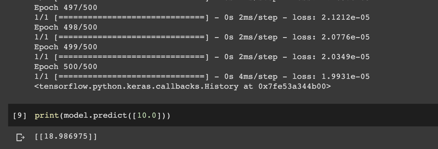
Here we can see get a value close to 19, but it's still off. There are two main reasons for this:
- We trained the model with a very small amount of data, only 6 points. So in this case there is a high probability the answer is 19, but the neural network isn't 100% sure.
- The other reason is that as neural networks try and figure out answers they deal in probabilities.
3. Introduction to Computer Vision
Now that we've looked at a simple example of machine learning, let's review a highly valuable application of this new programming paradigm: computer vision.
Computer vision is the field of AI that trains a computer to understand and label what's present in an image.
One way to teach a computer what's present in an image, for example different pieces of clothing, is with a dataset that has a large number of labelled images. Fortunately, the Fashion MNIST dataset has already done this for us, which includes:
- 70k images
- 10 categories
- Images are represented as a 28x28 array of greyscale
Let's now review how we can use this dataset to train a neural network.
Loading the Training Data
This data is actually preloaded into TensorFlow, so we can load it into our notebook as follows:
fashion_mnist = keras.datasets.fashion_mnist
(train_images, train_labels), (test_images, test_labels) = fashion_mnist.load_data()
As you can see, we separate some of the data into training sets and some into testing sets. In the Fashion MNIST dataset, 60k images are used for training and 10k are used for testing.
Building the Neural Network
Previously we had a neural network with one sequential layer, but now we have three layers:
- The first layer is a
Flattenlayer with input shape of 28x28, which turns it into a linear array. - The middle layer, also referred to as a hidden layer, has 128 neurons in it. You can think of these as variables in a function—there exists a set of these that turns the raw image data into the associated clothing class value.
- The last layer has 10 neurons because we have 10 classes of clothing.
model = keras.Sequential([
                          keras.layers.Flatten(input_shape=(28,28)),
                          keras.layers.Dense(128, activation=tf.nn.relu),
                          keras.layers.Dense(10, activation=tf.nn.softmax)])
We won't cover the full code for fashion MNIST in this article, although you can find an implementation in our guide on How to Build a Convolutional Neural Network in Python with Keras.
4. Introduction to Convolutional Neural Networks (CNNs)
We can take the simple deep neural network we just created for the Fashion MNIST dataset a step further with a specific type of network called a convolutional neural network.
As discussed in our article on What are Convolutional Neural Networks? A Guide to CNNs:
CNNs can look at images and identify spatial patterns such as shapes and colors. The shapes, colors, and anything else that distinguishes an image are called features. A CNN can learn to identify these features and use them for image classification.
Convolutions & Pooling
CNNs have convolutional layers and pooling layers. A convolutional layer is a technique to isolate features in an image. Pooling layers are a technique to reduce the information in images while maintaining features.
We can implement convolutional layers in TensorFlow with Conv2D and pooling layers with MaxPool2D, so we can extend our earlier code as follows:
model = tf.keras.models.Sequential([
                                    tf.keras.layers.Conv2D(64, (3,3), activation='relu',
                                                           input_shape=(28,28,1)),
                                    tf.keras.layers.MaxPooling2D(2,2),
                                    tf.keras.layers.Conv2D(64, (3,3), activation='relu'),
                                    tf.keras.layers.MaxPooling2D(2,2),
                                    tf.keras.layers.Flatten(),
                                    tf.keras.layers.Dense(128, activation='relu'),
                                    tf.keras.layers.Dense(10, activation='softmax')
])
You can learn more about computer vision and CNNs from this YouTube playlist from deeplearning.ai.
Introduction to ImageGenerator
We've now made our image classifier more efficient with convolutional and pooling layers, but it's still quite limited.
First off, all the images in the Fashion MNIST dataset are 28x28, in greyscale formate, and are perfectly centered. In the real-world, however, we're going to be dealing with more complex images that may not be formatted this perfectly.
That said, let's now look at how we can expand on our simple convolutational neural network to more complex images. As mentioned, real-world images will often include features in different locations and much larger images.
In the example below, we'll be classifying horses and humans, so it is binary classification. To deal with these complexities, the ImageGenerator API in TensorFlow can be very useful, which let's you:
Generate batches of tensor image data with real-time data augmentation.
For example, one feature of the API allows you to point it at a directory and the sub-directories will automatically generate labels for you.
Here's how we can use import this API in Keras:
from tensorflow.keras.preprocessing.image import ImageDataGeneratorWe can then instantiate ImageGenerator for our training directory as follows:
train_datagen = ImageDataGenerator(rescale=1./255)
train_generator = train_datagen.flow_from_directory(
    train_dir,
    target_size=(300,300),
    batch_size=128,
    class_mode='binary')
The other useful feature of this API is that the images are resized as they're loaded so you don't need to preprocess them beforehand.
ConvNet for More Complex Images
Here's the code to create a ConvNet that can classify horses and humans, which has a few key differences:
- There are three sets of convolutional layers at the top to reflect the increase complexity of the images.
- The output layer has one neuron because we're using the
sigmoidactivation function, which is useful for binary classification.
model = tf.keras.models.Sequential([
                                    tf.keras.layers.Conv2D(16, (3,3), activation='relu',
                                                           input_shape=(300,300,3)),
                                    tf.keras.layers.MaxPooling2D(2,2),
                                    tf.keras.layers.Conv2D(32,(3,3), activation='relu'),
                                    tf.keras.layers.MaxPooling2D(2,2),
                                    tf.keras.layers.Conv2D(64,(3,3), activation='relu'),
                                    tf.keras.layers.MaxPooling2D(2,2),
                                    tf.keras.layers.Flatten(),
                                    tf.keras.layers.Dense(512, activation='relu'),
                                    tf.keras.layers.Dense(1, activation='sigmoid')

])
Next we'll compile the model as follows:
from tensorflow.keras.optimizers import RMSprop
model.compile(loss='binary_crossentropy',
              optimizer=RMSprop(lr=0.001),
              metrics=['acc'])
Then we can train the model with fit_generator since we're using a generator instead of a dataset:
history = model.fit_generator(
    train_generator,
    steps_per_epoch=8,
    epochs=15,
    validation_data=validation_generator,
    validation_steps=8,
    verbose=2)
The final step is, of course, to perform some prediction with the model. We won't cover the full code for that in this article, although you can check out Week 4 of the Introduction to TensorFlow for Artificial Intelligence, Machine Learning, and Deep Learning for more details.
5. Convolutional Neural Networks for Larger Datasets
Now that we've reviewed building a basic convolutional neural network with TensorFlow, let's look at applying CNNs to much larger datasets. This section of the article is based on notes from course 2 of the specialization called Convolutional Neural Networks in TensorFlow.
One aspect of dealing with larger datasets is that there is less chance of overfitting, although it can still be an issue. In the next sections we'll look at how we can use data augmentation and transfer learning to reduce overfitting.
An example of a much larger dataset than we've seen so far is the famous Dogs vs. Cats dataset from Kaggle. As mentioned, with TensorFlow we can put our images into named subdirectories and ImageGenerator will automatically label them for us.
The model we can use is very similar to the one we just saw for Horses vs. Humans. Since it is so similar to what we just reviewed, we won't cover the notebook in this article, but you can find it on Github here.
6. Data Augmentation
Data augmentation is one of the most widely used tools to increase your dataset size and increase neural network performance. For example, in the Dogs vs. Cats dataset, we can diversify and augment the images by rotating, skewing, or transforming them.
There are a number of tools within TensorFlow to implement this, without losing data quality or overwriting the original data. You can learn more about data augmentation and the available transforms on the Keras preprocessing Github page.
One of the most important reasons for data augmentation is to avoid overfitting. In the context of convolutional neural networks, we pass convolutions over an image to learn particular features. By rotating an image, for example, we give the network more opportunity to learn which features classify the image, regardless of orientation. You can find the different Keras APIs for image augmentation here.
Here's an example of image augmentation with ImageDataGenerator:
train_datagen = ImageDataGenerator(
    rescale=1./255,
    rotation_range=40,
    width_shift_range=0.2,
    height_shift_range=0.2,
    shear_range=0.2,
    zoom_range=0.2,
    horizontal_flip=True,
    fill_mode='nearest'
)
7. Introduction to Transfer Learning
Transfer learning is another important technique in the field of deep learning. Instead of needing to train a neural network from scratch, we can download an open-source model that has already been trained and then use transfer learning to adapt it to our dataset.
In the context of convolutional neural networks, transfer learning allows us to take advantage of other models that have already been trained to extract features from much larger image datasets.
For example, we can use the convolutions already learned from a model such as the Inception Network, which has been trained on the ImageNet database that has over 1.4 million images and 1000 classes.
We can then retrain the dense layers and perhaps some of the lower convolutional layers from that model with our own data.
Fortunately, Keras has the Inception model built-in. Here's an example of how we load in the model with TensorFlow:
import os
from tensorflow.keras import layers
from tensorflow.keras import Model
from tensorflow.keras.applications.inception_v3 import InceptionV3
!wget --no-check-certificate \
    https://storage.googleapis.com/mledu-datasets/inception_v3_weights_tf_dim_ordering_tf_kernels_notop.h5 \
    -O /tmp/inception_v3_weights_tf_dim_ordering_tf_kernels_notop.h5
local_weights_file = '/tmp/inception_v3_weights_tf_dim_ordering_tf_kernels_notop.h5'
pre_trained_model = InceptionV3(input_shape = (150, 150, 3),
                                include_top = False,
                                weights = None)
pre_trained_model.load_weights(local_weights_file)
pre_trained_model.summary()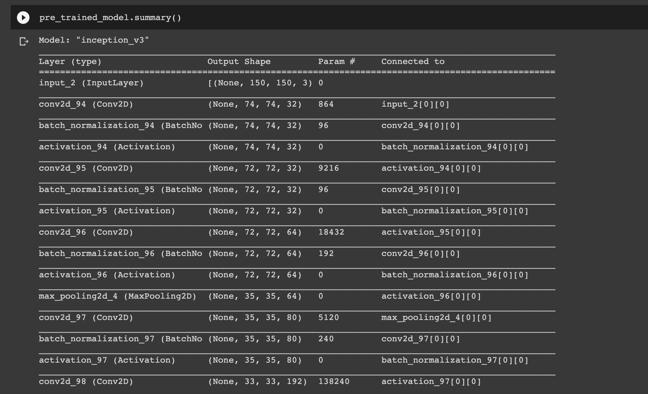
You can a transfer learning tutorial on how to freeze or lock convolutional layers with TensorFlow here.
8. Multi-class Classification
We've been reviewing binary classification problems, although many real-world applications will require more than two outputs.
In this section, we'll discuss important coding differences between multi-class and binary classifiers. In particular, we'll look at how TensorFlow's ImageGenerator works for multi-class classification.
In order to use ImageGenerator with 3 subclasses all we need to do is set up 3 subdirectories within our Training and Validation folders. For example, we can use the Rock Paper Scissors dataset by Laurence Moroney, which contains 2892 images of diverse hands in Rock/Paper/Scissors poses.
To deal with multiple classes, we can simply change our class_mode to categorical as follows:
train_datagen = ImageDataGenerator(rescale=1./255)
train_generator = train_datagen.flow_from_directory(
    train_dir,
    target_size=(300,300),
    batch_size=128,
    class_mode='categorical')
We'll also need to change the output of our model's activation from sigmoid to softmax, which will return the probability of each class that an image represents:
model = tf.keras.models.Sequential([
                                    tf.keras.layers.Conv2D(16, (3,3), activation='relu',
                                                           input_shape=(300,300,3)),
                                    tf.keras.layers.MaxPooling2D(2,2),
                                    tf.keras.layers.Conv2D(32,(3,3), activation='relu'),
                                    tf.keras.layers.MaxPooling2D(2,2),
                                    tf.keras.layers.Conv2D(64,(3,3), activation='relu'),
                                    tf.keras.layers.MaxPooling2D(2,2),
                                    tf.keras.layers.Flatten(),
                                    tf.keras.layers.Dense(512, activation='relu'),
                                    tf.keras.layers.Dense(1, activation='softmax')

])
Finally, when we're compiling our model we'll need to change our loss from binary_crossentropy to categorical_crossentropy:
from tensorflow.keras.optimizers import RMSprop
model.compile(loss='categorical_crossentropy',
              optimizer=RMSprop(lr=0.001),
              metrics=['acc'])
Summary: TensorFlow for Convolutional Neural Networks (CNNs)
As discussed in this article, we can go from a simple deep neural network to more complex convolutional neural networks with relatively few lines of code using TensorFlow.
Convolutional neural networks use various layers to extract features from an image, which can then be used for classification. One of the main issues we'll encounter with CNNs is overfitting to the data, although we can use tools such as Image Augmentation and Transfer Learning to avoid this. Below, you'll find additional resources for TensorFlow, computer vision, and convolutional neural networks.

