Time Series with TensorFlow: Building a multivariate time series forecasting model

In this Time Series with TensorFlow article, we create a multivariate dataset, prepare it for modeling, and then create a simple dense model for forecasting.

a year ago • 7 min read

By Peter Foy

As we saw in previous articles in this Time Series with TensorFlow series, all of our deep learning models have not yet outperformed our naive model.

In all of our previous models, we've been using price as the only input, in other words, we've been using univariate time series data.

In this article, we're going to turn our data from univariate into a multivariate time series dataset, which means it consists of two or more variables (features).

This article is based on notes from this TensorFlow Developer Certificate course and is organized as follows:

How to turn our univariate time series into multivariate
Preparing our multivariate time series for a model
Model 6: Building a model for multivariate time series data

Previous articles in this series can be found below:

Stay up to date with AI

How to turn our univariate time series into multivariate

Before we add features to our dataset, let's first consider what we could use. As you can imagine, there's a nearly limitless amount of data that could influence the price of Bitcoin, a few examples of which include:

Bitcoin mining difficulty
Bitcoin halving events
News sentiment
Daily volume
And so on

For now, let's look at how we could add bitcoin halving events (i.e. block rewards) to our dataset.

Since there aren't many of these events, we can add them manually. Note, since our price dataset doesn't start until 2014, we won't see the first halving event in our dataset.

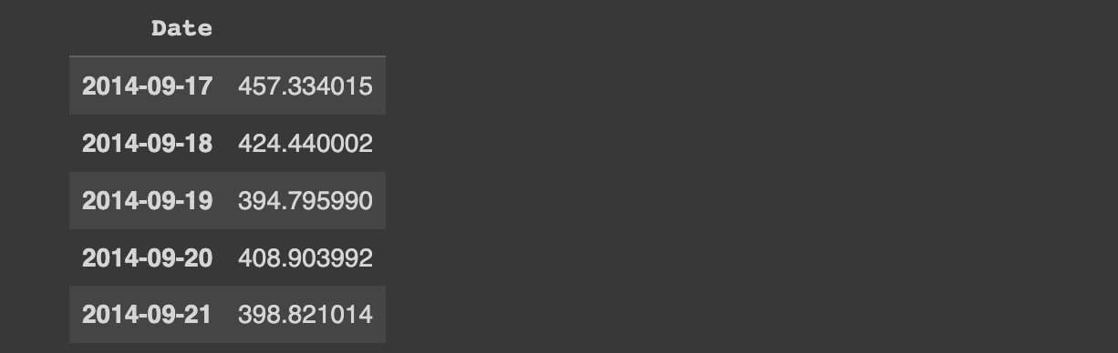
Let's add the block reward and dates to our dataset as follows:

# Let's add halving events to our dataset
block_reward_1 = 50 # 3 Jan 2009 - this block reward isn't in our dataset
block_reward_2 = 25 # 28 Nov 2012 - also not in our dataset
block_reward_3 = 12.5 # 9 July 2016
block_reward_4 = 6.25 # 18 May 2020

# Block reward dates
block_reward_2_datetime = np.datetime64("2012-11-28")
block_reward_3_datetime = np.datetime64("2016-07-09")
block_reward_4_datetime = np.datetime64("2020-05-18")

Next, we need to add this data into our existing dataset. One way to do that is to get the date indexes where we should add the halving event.

This means we'll need to create ranges between each of the halving events so we can assign the value of the block reward size.

First, let's create date ranges of where specific block_reward values should be. Since we have our block_reward_2_datetime as an np.datetime64 value, we can use this on the index of our bitcoin price data as follows:

# Create date ranges to assign block_reward values
block_reward_2_days = (block_reward_3_datetime - bitcoin_prices.index[0]).days
block_reward_2_days

What this is saying is to get all the days from 9 July 2016 to the first index of our price data. Let's now do the same for block_reward_3_days

# Create date ranges to assign block_reward values
block_reward_2_days = (block_reward_3_datetime - bitcoin_prices.index[0]).days
block_reward_3_days = (block_reward_4_datetime - bitcoin_prices.index[0]).days
block_reward_2_days, block_reward_3_days

(661, 2070)

Now we can see everything up until index 661 will be block_reward_2 and everything between index 661 and 20270 will be block_reward_3.

Let's now add in a block_reward column:

# Add in a block_reward column
bitcoin_prices_block = bitcoin_prices.copy()
bitcoin_prices_block["block_reward"] = None

We'll then add in block_reward values as a feature to our dataframe:

# Add in block_reward values as a feature to our dataframe
bitcoin_prices_block.iloc[:block_reward_2_days, -1] = block_reward_2
bitcoin_prices_block.iloc[block_reward_2_days:block_reward_3_days, -1] = block_reward_3
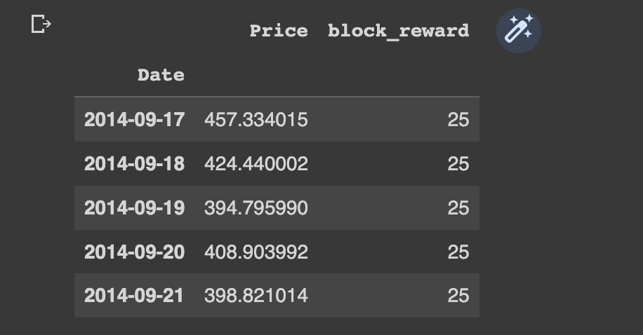
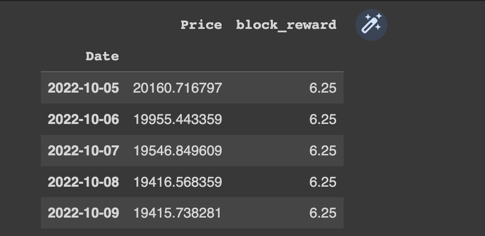
bitcoin_prices_block.iloc[block_reward_3_days:, -1] = block_reward_4

Now we can see the head and tail of our dataframe have the block reward as a column:

If we try and plot our new multivariate dataframe as is, we see they're on different scales so we don't get much value from the image:

bitcoin_prices_block.plot(figsize=(10,7));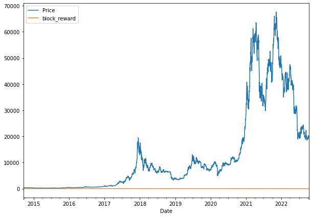

In order to plot these on the same image let's adjust their scale with sklearn's minmax_scale preprocessing function as follows:

# Plot the block reward vs. price over time
from sklearn.preprocessing import minmax_scale
scaled_price_block_df = pd.DataFrame(minmax_scale(bitcoin_prices_block[['Price', 'block_reward']]),
                                     columns=bitcoin_prices_block.columns,
                                     index=bitcoin_prices_block.index)

scaled_price_block_df.plot(figsize=(10,7));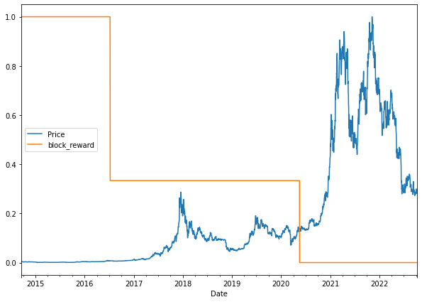

Now that we have a multivariate time series dataset, let's prepare it for model building.

Preparing our multivariate time series for a model

Before we build our next model, we need to prepare the multivariate data as a windowed dataset.

We had previously created the helper function make_windows() for this purpose, although it is only for univariate data.

Since our multivariate dataset is in a dataframe, we're going to use Pandas to create our windows. Specifically, we'll use the pandas.DataFrame.shift() method to window our multivariate data - you can learn more about it here.

First, let's set up our dataset hyperparameters:

# Setup dataset hyperparameters
HORIZON = 1
WINDOW_SIZE = 7

To use the shift function, next we're going to make a copy of our Bitcoin historical data with the block reward feature. We'll then add our windowed columns as follows:

# Make a copy of Bitcoin historical data with block reward feature
bitcoin_prices_windowed = bitcoin_prices_block.copy()

# Add windowed columns
for i in range(WINDOW_SIZE): # shift value for each step in WINDOW_SIZE
  bitcoin_prices_windowed[f"Price+{i+1}"] = bitcoin_prices_windowed["Price"].shift(periods=i+1)
bitcoin_prices_windowed.head(10)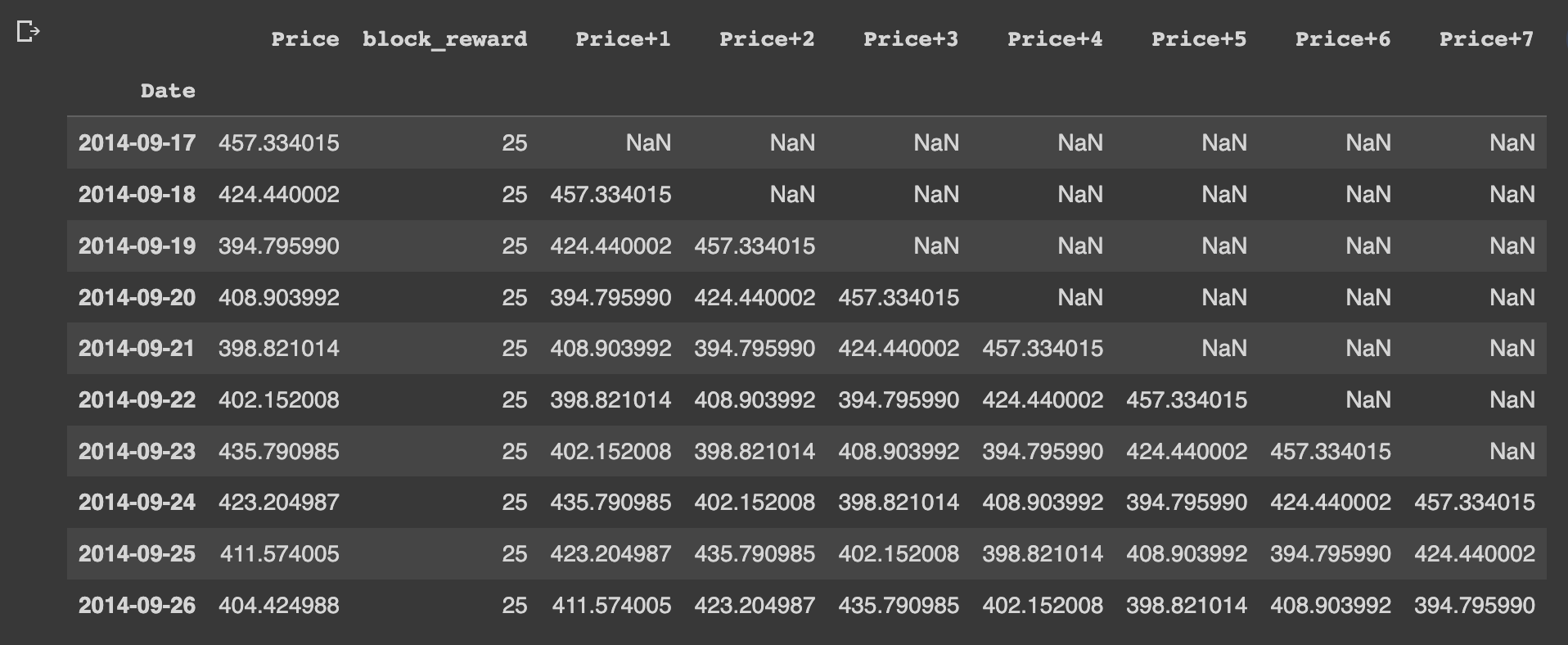

What this means is that the horizon for the 7 windowed values (block_reward, Price+1, Price+2, etc.) will be the Price column.

Lets now create X windows and y horizon features:

X = bitcoin_prices_windowed.dropna().drop("Price", axis=1).astype(np.float32)
y = bitcoin_prices_windowed.dropna()["Price"].astype(np.float32)

Before we can pass this time series data to a model, the last thing to do is split it into train and test sets.

We can split our data into train and test sets using indexing as follows:

# Split into train and test sets using indexing
split_size = int(len(X) * 0.8)
X_train, y_train = X[:split_size], y[:split_size] 
X_test, y_test = X[split_size:], y[split_size:]
len(X_train), len(y_train), len(X_test), len(y_test)

Model 6: Building a model for multivariate time series data

Now that we have our multivariate data prepared for model building, let's create a simple dense model similar to model_1, which is summarized below:

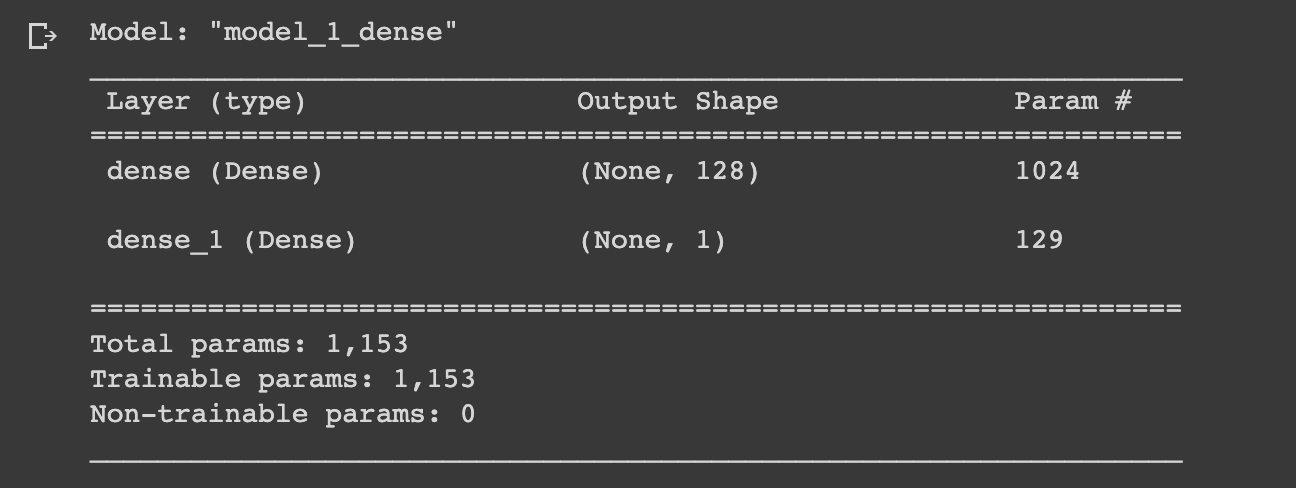
Let's recreate this model but for multivariate time series data. Note, we actually don't need to change the model architecture at all for it to work since it's just our input data that is different:

# Model 6: Multivariate time series
tf.random.set_seed(42)

# Build model
model_6 = tf.keras.Sequential([
    layers.Dense(128, activation="relu"),
    layers.Dense(HORIZON)
], name="model_6_dense_multivariate")

# Compile model
model_6.compile(loss="mae",
                optimizer=tf.keras.optimizers.Adam())

# Fit model
model_6.fit(X_train, y_train,
            epochs=100,
            verbose=1,
            validation_data=(X_test, y_test),
            callbacks=[create_model_checkpoint(model_name=model_6.name)])

Let's now evaluate the multivariate model against our previous univariate models, to do so we'll:

Evaluate the multivariate model
Load in the best performing model
Make predictions with the model
Evaluate predictions with our evaluation metrics

# Evalutate multivariate model
model_6.evaluate(X_test, y_test)

# Load in and evaluate best performing model
model_6 = tf.keras.models.load_model("model_experiments/model_6_dense_multivariate")
model_6.evaluate(X_test, y_test)

# Make predictions with multivariate model
model_6_preds = tf.squeeze(model_6.predict(X_test))
model_6_preds[:10]

# Evaluate predictions to get eval metrics
model_6_results = evaluate_preds(y_true=y_test,
                                 y_pred=model_6_preds)
model_6_results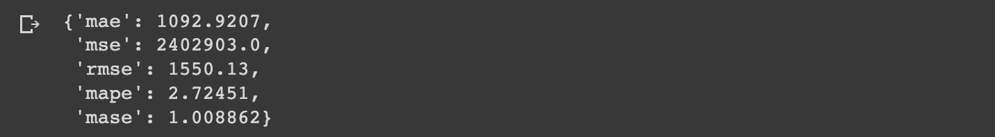

Let's now compare these results to previous models and our naive results:

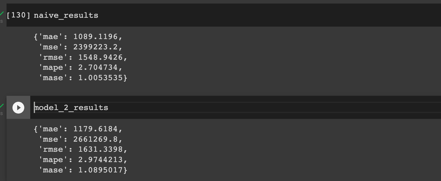
As we can see, we're now very close to our naive results and slightly better than our univariate dense model.

Summary: Building a multivariate time series forecasting model

In this article, we saw how we can add a feature to our data in order to change it from a univariate dataset to a multivariate dataset.

We then discussed how we can prepare this multivariate data for modeling by creating a windowed dataset with the Pandas shift function.

Finally, we recreated our first dense model with multivariate data and saw a slight improvement from previous models.

Keep in mind this is still a very simple model, so in the next article, we'll expand on this and use our multivariate data to build the N-BEATS algorithm.